


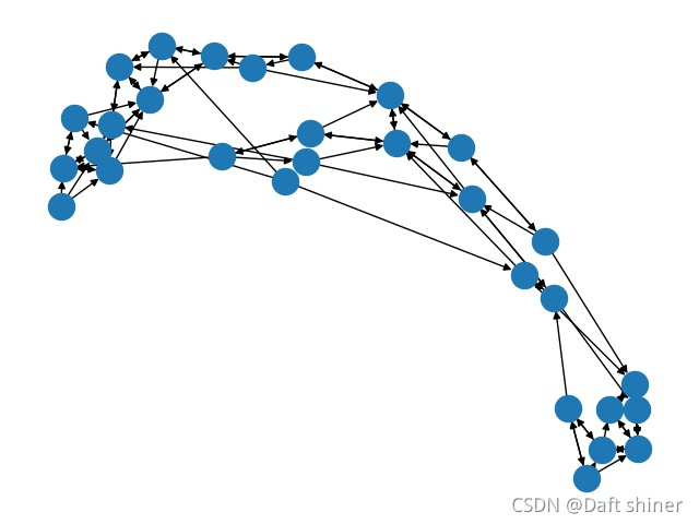
 博客介绍了如何在没有现成库支持的情况下,手动计算网络指标并可视化加权有向图。使用NetworkX库尝试了多种节点布局,包括random_layout、circular_layout、shell_layout、spring_layout、spectral_layout和kamada_kawai_layout。作者提供了代码示例,但未提供具体数据,建议读者使用自定义邻接矩阵进行尝试。最后,博主遇到了标签和节点重叠的可视化问题,并展示了部分可视化结果。
最近在做的东西需要可视化加权有向图,从前做惯了无脑调包的无权无向图,现在不仅网络指标全部得自己算,网络的可视化也是个大问题,在此写下此博客记录自己的学习过程。
Graph Layout
先看节点布局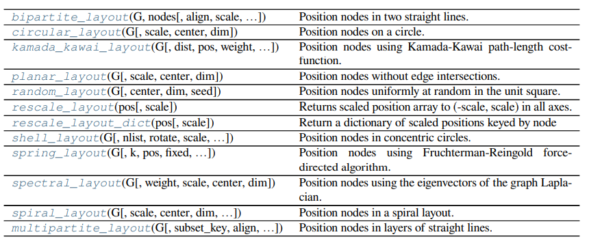
这里只是对每种布局有所了解,且由于这里是本人用私有数据得到的加权有向图(节点数30)可视化的,这里就不公布文件了,大家可以随机生成一个邻接矩阵进行可视化操作。
pos = nx.random_layout(G)
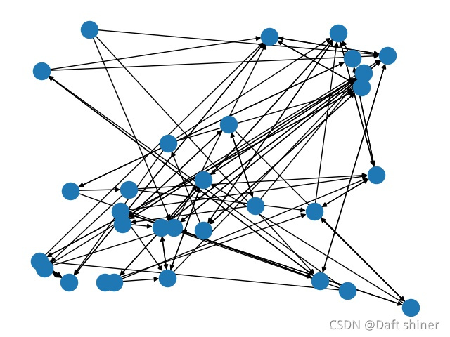
pos = nx.circular_layout(G)
pos = nx.shell_layout(G)

pos = nx.spring_layout(G)
pos = nx.spectral_layout(G)
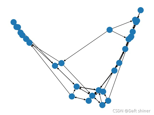
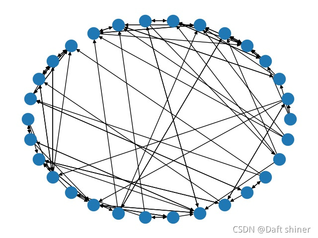
pos = nx.kamada_kawai_layout(G)
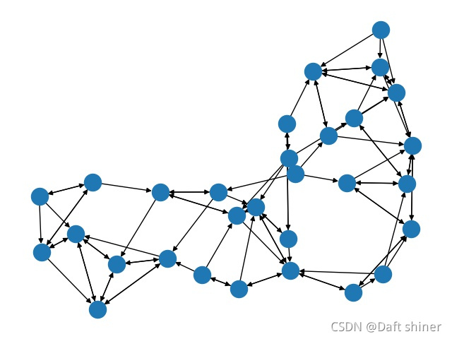
pos = nx.spiral_layout(G)
 最低0.47元/天 解锁文章


 3031
3031

 被折叠的 条评论
为什么被折叠?
被折叠的 条评论
为什么被折叠?
 到【灌水乐园】发言


