python绘制海底地形图（海底高程图）（3D绘图+三种插值法实践）

表：海底水深数据

x	129	140	103.5	88	185.5	195	105	157.5	107.5	77	81	162	162	117.5
y	7.5	141.5	23	147	22.5	137.5	85.5	-6.5	-81	3	56.5	-66.5	84	-33.5
z	4	8	6	8	6	8	8	9	9	8	8	9	4	9

注：数据来自《数学建模算法与应用（第2版）》，p91，司守奎，孙兆亮，国防工业出版社，2020.2重印

import numpy as np
points = np.array([129,140,103.5,88,185.5,195,105,157.5,107.5,77,81,162,162,117.5,7.5,141.5,23,
147,22.5,137.5,85.5,-6.5,-81,3,56.5,-66.5,84,-33.5]).reshape(14,2)  
#这是给定数据的(xi, yi)，只是先输入了全部x又输入了全部y
values = np.array([-4,-8,-6,-8,-6,-8,-8,-9,-9,-8,-8,-9,-4,-9])  #这是给定数据的zi

grid_x, grid_y = np.mgrid[0:200:400j, -100:200:600j] #这是插值点的(xi,yi)
from scipy.interpolate import griddata            #这是求插值点的zi
grid_z0 = griddata(points, values, (grid_x, grid_y), method='nearest')
grid_z1 = griddata(points, values, (grid_x, grid_y), method='linear')
grid_z2 = griddata(points, values, (grid_x, grid_y), method='cubic')

#下面是绘图
import matplotlib.pyplot as plt
from mpl_toolkits.mplot3d.axes3d import Axes3D
plt.figure()

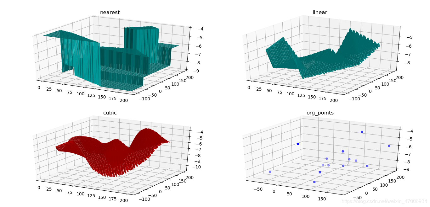
ax1 = plt.subplot2grid((2,2), (0,0), projection='3d')
ax1.plot_surface(grid_x, grid_y, grid_z0, color = "c")
ax1.set_title('nearest')

ax2 = plt.subplot2grid((2,2), (0,1), projection='3d')
ax2.plot_surface(grid_x, grid_y, grid_z1, color = "c")
ax2.set_title('linear')

ax3 = plt.subplot2grid((2,2), (1,0), projection='3d')
ax3.plot_surface(grid_x, grid_y, grid_z2, color = "r")
ax3.set_title('cubic')

ax4 = plt.subplot2grid((2,2), (1,1), projection='3d')
ax4.scatter(points[:,0], points[:,1], values,  c= "b")
ax4.set_title('org_points')

plt.tight_layout()
plt.show()

 以下是三种插值方法+原数据绘图的结果：

附：一个解析明确的参考文档：http://liao.cpython.org/scipytutorial11/

最后作者想说的是：和matlab插值还是差很多，只可惜matlab输出的图片样式实在是充满了年代感。。