


8. This question involves the use of simple linear regression on the Auto data set.
(a) Use the lm() function to perform a simple linear regression with mpg as the response and horsepower as the predictor. Use the summary() function to print the results. Comment on the output.
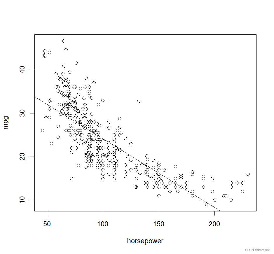
There is a negative relationship between the response and the predictor at the 0.1% significance level. When the predictor horsepower increases by one unit, the response mpg will decrease by 0.158 units. The relationship between them is negative.
The predicted mpg associated with a horsepower of 98 is 24.46708. The 95% confidence interval associated with a horsepower value of 98 is (23.97, 24.96), and the 95% prediction interval is (14.81, 34.12).
1.	>attach(Auto)
2.	> str(auto)
3.	> View(auto)
4.	> lm.1<-lm(mpg~horsepower,data=Auto)
5.	> View(lm.1)
6.	> summary(lm.1)
7.
8.	Call:
9.	lm(formula = mpg ~ horsepower, data = Auto)
10.
11.	Residuals:
12.	     Min       1Q   Median       3Q      Max
13.	-13.5710  -3.2592  -0.3435   2.7630  16.9240
14.
15.	Coefficients:
16.	             Estimate Std. Error t value Pr(>|t|)
17.	(Intercept) 39.935861   0.717499   55.66   <2e-16 ***
18.	horsepower  -0.157845   0.006446  -24.49   <2e-16 ***
19.	---
20.	Signif. codes:  0 ‘***’ 0.001 ‘**’ 0.01 ‘*’ 0.05 ‘.’ 0.1 ‘ ’ 1
21.
22.	Residual standard error: 4.906 on 390 degrees of freedom
23.	Multiple R-squared:  0.6059, Adjusted R-squared:  0.6049
24.	F-statistic: 599.7 on 1 and 390 DF,  p-value: < 2.2e-16
25.
26.	> predict(lm.1,data.frame(horsepower=c(98)),interval="confidence")
27.	       fit      lwr      upr
28.	1 24.46708 23.97308 24.96108
29.	> predict(lm.1,data.frame(horsepower=c(98)),interval="prediction")
30.	       fit     lwr      upr
31.	1 24.46708 14.8094 34.12476
32.	>
(b) Plot the response and the predictor. Use the abline() function to display the least squares regression line.
The picture is shown below.
(c) Use the plot() function to produce diagnostic plots of the least squares regression fit. Comment on any problems you see with the fit.
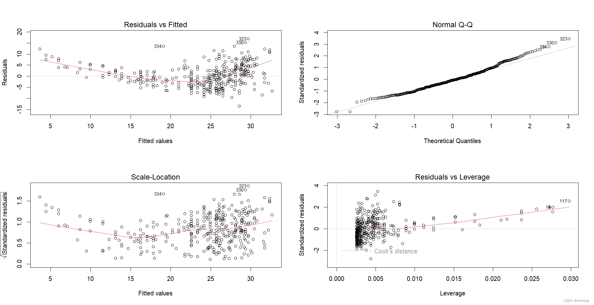
It can be seen from the scatter plot of residual term and fitting value that there may be a curve-like relationship between them, indicating that a quadratic term of the independent variable might be needed in the original regression model.
10. This question should be answered using the Carseats data set.
(a) Fit a multiple regression model to predict Sales using Price, Urban, and US.
1.	> attach(Carseats)
2.	The following objects are masked from Carseats (pos = 3):
3.
4.	    Advertising, Age, CompPrice, Education, Income, Population, Price, Sales, ShelveLoc, Urban, US
5.
6.	> lm.10<-lm(Sales~Price+Urban+US)
7.	> summary(lm.10)
8.
9.	Call:
10.	lm(formula = Sales ~ Price + Urban + US)
11.
12.	Residuals:
13.	    Min      1Q  Median      3Q     Max
14.	-6.9206 -1.6220 -0.0564  1.5786  7.0581
15.
16.	Coefficients:
17.	             Estimate Std. Error t value Pr(>|t|)
18.	(Intercept) 13.043469   0.651012  20.036  < 2e-16 ***
19.	Price       -0.054459   0.005242 -10.389  < 2e-16 ***
20.	UrbanYes    -0.021916   0.271650  -0.081    0.936
21.	USYes        1.200573   0.259042   4.635 4.86e-06 ***
22.	---
23.	Signif. codes:  0 ‘***’ 0.001 ‘**’ 0.01 ‘*’ 0.05 ‘.’ 0.1 ‘ ’ 1
24.
25.	Residual standard error: 2.472 on 396 degrees of freedom
26.	Multiple R-squared:  0.2393, Adjusted R-squared:  0.2335
27.	F-statistic: 41.52 on 3 and 396 DF,  p-value: < 2.2e-16
(b) Provide an interpretation of each coefficient in the model. Be careful-some of the variables in the model are qualitative!
The first coefficient is 13.043469, which is the intercept term.
The second is the coefficient of Price, which means that when other conditions are held constant, the sales volume will decrease by 0.054 units for each unit increase in price.
The third coefficient indicates that the sales volume of stores in cities is 0.022 units lower than the sales volume of stores outside cities.
The fourth coefficient indicates that the sales volume of stores in US is 1.201 units higher than the sales volume of stores outside the US.
(c) Write out the model in equation form, being careful to handle the qualitative variables properly.
Sales=13.043469-0.054459*Price-0.021916*Urban+1.200583*US+e
When the store is in the urban area in US, Sales=14.222136-0.054459*Price+e
When the store is in the urban area but not in US, Sales=13.021553-0.054459*Price+e
When the store is not in the urban area but in US, Sales=14.244052-0.054459*Price+e
When the store is not in the urban area and not in US, Sales=13.043469-0.054459*Price+e
(d) For which of the predictors can you reject the null hypothesis H0 : βj = 0?
Price and US.
(e) On the basis of your response to the previous question, fit a smaller model that only uses the predictors for which there is evidence of association with the outcome.
1.	> lm.10e<-lm(Sales~Price+US)
2.	> summary(lm.10e)
3.
4.	Call:
5.	lm(formula = Sales ~ Price + US)
6.
7.	Residuals:
8.	    Min      1Q  Median      3Q     Max
9.	-6.9269 -1.6286 -0.0574  1.5766  7.0515
10.
11.	Coefficients:
12.	            Estimate Std. Error t value Pr(>|t|)
13.	(Intercept) 13.03079    0.63098  20.652  < 2e-16 ***
14.	Price       -0.05448    0.00523 -10.416  < 2e-16 ***
15.	USYes        1.19964    0.25846   4.641 4.71e-06 ***
16.	---
17.	Signif. codes:  0 ‘***’ 0.001 ‘**’ 0.01 ‘*’ 0.05 ‘.’ 0.1 ‘ ’ 1
18.
19.	Residual standard error: 2.469 on 397 degrees of freedom
20.	Multiple R-squared:  0.2393, Adjusted R-squared:  0.2354
21.	F-statistic: 62.43 on 2 and 397 DF,  p-value: < 2.2e-16
(f) How well do the models in (a) and (e) fit the data?
Compare the adjusted R-squared. The adjusted R-squared in model (a) is 0.2335 while the adjusted R-squared in model (e) is 0.2354, which means model (e) fits the data better and can explain 23.54% of the variation in the dependent variable.
(g) Using the model from (e), obtain 95% confidence intervals for the coefficient(s).
1.	confint(lm.10e,level=0.95)
2.	                  2.5 %      97.5 %
3.	(Intercept) 11.79032020 14.27126531
4.	Price       -0.06475984 -0.04419543
5.	USYes        0.69151957  1.70776632
The 95% confidence intervals for Price is [-0.065, -0.044] and the 95% confidence intervals for US is [0.692, 1.708].
(h) Is there evidence of outliers or high leverage observations in the model from (e)?
Outliers:
Residual plots can be used to identify outliers. Plot the studentized residuals and we can find that all the observations have studentized residuals between-3 and 3, which means no outliers are suggested in the model (e).
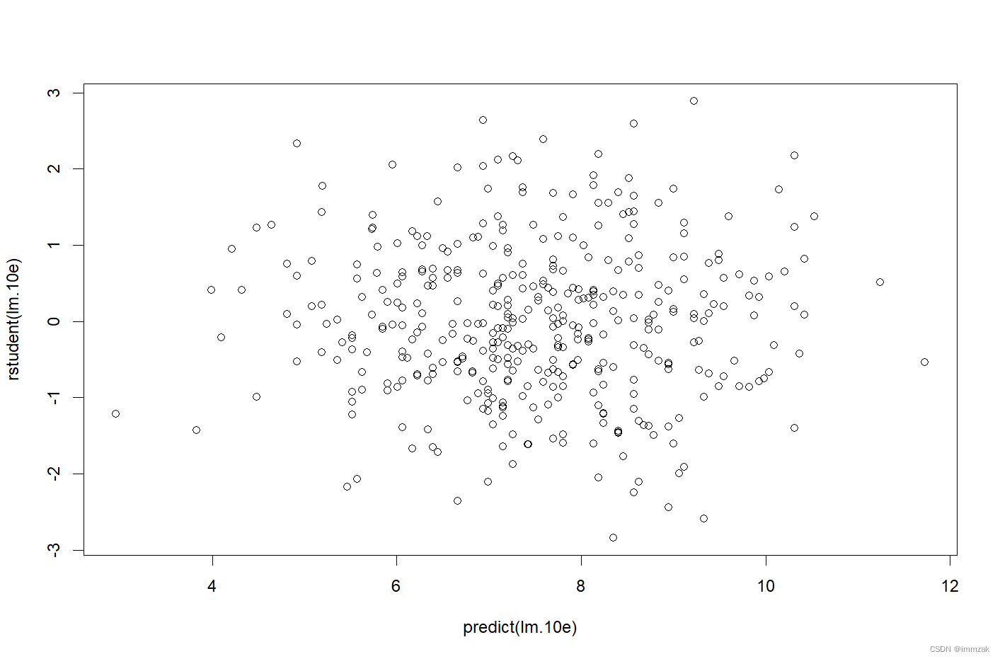
High leverage:
After drawing the leverage-statistic plot, it is found that some observations have high leverage. Among them, the observation 43 have the highest leverage statistics.
1.	> par(mfrow=c(2,2))
2.	> plot(lm.10e)
3.	> plot(hatvalues(lm.10e))
4.	> which.max(hatvalues(lm.10e))
5.	43
6.	43
![]()
12. This problem involves simple linear regression without an intercept.
(a) Recall that the coefficient estimate β![]() for the linear regression of Y onto X without an intercept is given by (3.38). Under what circumstance is the coefficient estimate for the regression of X onto Y the same as the coefficient estimate for the regression of Y onto X?
for the linear regression of Y onto X without an intercept is given by (3.38). Under what circumstance is the coefficient estimate for the regression of X onto Y the same as the coefficient estimate for the regression of Y onto X?
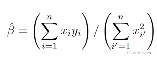
According to the formula 3.38 (shown below), when , the coefficient estimates are the same.
(b) Generate an example in R with n = 100 observations in which the coefficient estimate for the regression of X onto Y is different from the coefficient estimate for the regression of Y onto X.
1.	> set.seed(1)
2.	> x = rnorm(100)
3.	> y = 3*x
4.	> lm.12b1= lm(y~x+0)
5.	> lm.12b2 = lm(x~y+0)
6.	> summary(lm.12b1)
7.
8.	Call:
9.	lm(formula = y ~ x + 0)
10.
11.	Residuals:
12.	       Min         1Q     Median         3Q        Max
13.	-8.558e-16 -4.290e-17  4.600e-18  1.410e-16  1.173e-14
14.
15.	Coefficients:
16.	   Estimate Std. Error   t value Pr(>|t|)
17.	x 3.000e+00  1.334e-16 2.249e+16   <2e-16 ***
18.	---
19.	Signif. codes:  0 ‘***’ 0.001 ‘**’ 0.01 ‘*’ 0.05 ‘.’ 0.1 ‘ ’ 1
20.
21.	Residual standard error: 1.201e-15 on 99 degrees of freedom
22.	Multiple R-squared:      1, Adjusted R-squared:      1
23.	F-statistic: 5.059e+32 on 1 and 99 DF,  p-value: < 2.2e-16
24.
25.	Warning message:
26.	In summary.lm(lm.12b1) : essentially perfect fit: summary may be unreliable
27.	> summary(lm.12b2)
28.
29.	Call:
30.	lm(formula = x ~ y + 0)
31.
32.	Residuals:
33.	       Min         1Q     Median         3Q        Max
34.	-2.624e-15 -4.547e-17 -3.270e-18  3.747e-17  2.846e-16
35.
36.	Coefficients:
37.	   Estimate Std. Error   t value Pr(>|t|)
38.	y 3.333e-01  1.022e-17 3.261e+16   <2e-16 ***
39.	---
40.	Signif. codes:  0 ‘***’ 0.001 ‘**’ 0.01 ‘*’ 0.05 ‘.’ 0.1 ‘ ’ 1
41.
42.	Residual standard error: 2.761e-16 on 99 degrees of freedom
43.	Multiple R-squared:      1, Adjusted R-squared:      1
44.	F-statistic: 1.064e+33 on 1 and 99 DF,  p-value: < 2.2e-16
45.
46.	Warning message:
47.	In summary.lm(lm.12b2) : essentially perfect fit: summary may be unreliable
(c) Generate an example in R with n = 100 observations in which the coefficient estimate for the regression of X onto Y is the same as the coefficient estimate for the regression of Y onto X.
1.	> set.seed(1)
2.	> x=rnorm(100)
3.	> y=-sample(x, 100)
4.	> sum(x^2)
5.	[1] 81.05509
6.	> sum(y^2)
7.	[1] 81.05509
8.	> lm.12c1 <- lm(y~x+0)
9.	> lm.12c2 <- lm(x~y+0)
10.	> summary(lm.12c1)
11.
12.	Call:
13.	lm(formula = y ~ x + 0)
14.
15.	Residuals:
16.	    Min      1Q  Median      3Q     Max
17.	-2.2833 -0.6945 -0.1140  0.4995  2.1665
18.
19.	Coefficients:
20.	  Estimate Std. Error t value Pr(>|t|)
21.	x  0.07768    0.10020   0.775     0.44
22.
23.	Residual standard error: 0.9021 on 99 degrees of freedom
24.	Multiple R-squared:  0.006034, Adjusted R-squared:  -0.004006
25.	F-statistic: 0.601 on 1 and 99 DF,  p-value: 0.4401
26.
27.	> summary(lm.12c2)
28.
29.	Call:
30.	lm(formula = x ~ y + 0)
31.
32.	Residuals:
33.	    Min      1Q  Median      3Q     Max
34.	-2.2182 -0.4969  0.1595  0.6782  2.4017
35.
36.	Coefficients:
37.	  Estimate Std. Error t value Pr(>|t|)
38.	y  0.07768    0.10020   0.775     0.44
39.
40.	Residual standard error: 0.9021 on 99 degrees of freedom
41.	Multiple R-squared:  0.006034, Adjusted R-squared:  -0.004006
42.	F-statistic: 0.601 on 1 and 99 DF,  p-value: 0.4401
14.This problem focuses on the collinearity problem.
(a) Perform the following commands in R:
> set.seed(1)
> x1=runif (100)
> x2=0.5*x1+rnorm (100)/10
> y=2+2*x1+0.3*x2+rnorm (100)
The last line corresponds to creating a linear model in which y is a function of x1 and x2. Write out the form of the linear model. What are the regression coefficients?
The form of the linear model is: y=2+2*x1+0.3*x2+e
The regression coefficients are: β0=2, β1=2, β3=0.3
(b) What is the correlation between x1 and x2? Create a scatterplot displaying the relationship between the variables.
The correlation between x1 and x2 is 0.8351212.
1.	> cor(x1,x2)
2.	[1] 0.8351212
3.	> plot(x1,x2)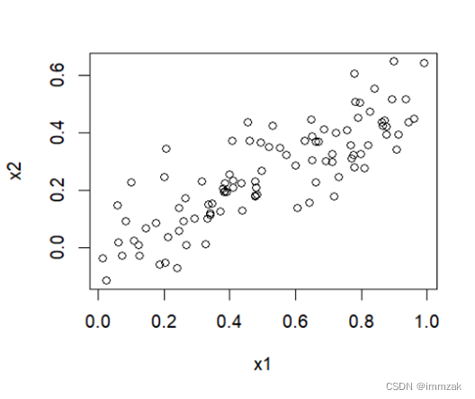
(c) Using this data, fit a least squares regression to predict y using x1 and x2. Describe the results obtained. What are![]() ,
, ![]() ,and
,and![]() ? How do these relate to the true β0, β1, and β2? Can you reject the null hypothesis H0 : β1= 0? How about the null hypothesis H0 : β2= 0?
? How do these relate to the true β0, β1, and β2? Can you reject the null hypothesis H0 : β1= 0? How about the null hypothesis H0 : β2= 0?
1.	> lm.14c = lm(y~x1+x2)
2.	> summary(lm.14c)
3.
4.	Call:
5.	lm(formula = y ~ x1 + x2)
6.
7.	Residuals:
8.	    Min      1Q  Median      3Q     Max
9.	-2.8311 -0.7273 -0.0537  0.6338  2.3359
10.
11.	Coefficients:
12.	            Estimate Std. Error t value Pr(>|t|)
13.	(Intercept)   2.1305     0.2319   9.188 7.61e-15 ***
14.	x1            1.4396     0.7212   1.996   0.0487 *
15.	x2            1.0097     1.1337   0.891   0.3754
16.	---
17.	Signif. codes:  0 ‘***’ 0.001 ‘**’ 0.01 ‘*’ 0.05 ‘.’ 0.1 ‘ ’ 1
18.
19.	Residual standard error: 1.056 on 97 degrees of freedom
20.	Multiple R-squared:  0.2088, Adjusted R-squared:  0.1925
21. F-statistic: 12.8 on 2 and 97 DF, p-value: 1.164e-05![]() =2.1305
=2.1305
![]() =1.4396
=1.4396
![]() =1.0097
=1.0097
According to the p-value, the p-value of the intercept is below 0.001, which indicates that ![]() is quite close to the true
is quite close to the true ![]() . The p-value of x2 is above 0.1, which indicates that
. The p-value of x2 is above 0.1, which indicates that ![]() is not close to true
is not close to true![]() .
.
We can reject the null hypothesis for β1 because the p-value of β1 is below 0.05. We cannot reject the null hypothesis for β2 because the p-value of β2 is above 0.1 indicating that the coefficient is not significant.
(d) Now fit a least squares regression to predict y using only x1. Comment on your results. Can you reject the null hypothesis H0 : β1= 0?
1.	> lm.14d = lm(y~x1)
2.	> summary(lm.14d)
3.
4.	Call:
5.	lm(formula = y ~ x1)
6.
7.	Residuals:
8.	     Min       1Q   Median       3Q      Max
9.	-2.89495 -0.66874 -0.07785  0.59221  2.45560
10.
11.	Coefficients:
12.	            Estimate Std. Error t value Pr(>|t|)
13.	(Intercept)   2.1124     0.2307   9.155 8.27e-15 ***
14.	x1            1.9759     0.3963   4.986 2.66e-06 ***
15.	---
16.	Signif. codes:  0 ‘***’ 0.001 ‘**’ 0.01 ‘*’ 0.05 ‘.’ 0.1 ‘ ’ 1
17.
18.	Residual standard error: 1.055 on 98 degrees of freedom
19.	Multiple R-squared:  0.2024, Adjusted R-squared:  0.1942
20.	F-statistic: 24.86 on 1 and 98 DF,  p-value: 2.661e-06
We reject the null hypothesis H0 : β1= 0 because the p-value of x1 is below 0.001.
(e) Now fit a least squares regression to predict y using only x2. Comment on your results. Can you reject the null hypothesis H0 : β1 = 0?
1.	> lm.14e= lm(y~x2)
2.	> summary(lm.14e)
3.
4.	Call:
5.	lm(formula = y ~ x2)
6.
7.	Residuals:
8.	     Min       1Q   Median       3Q      Max
9.	-2.62687 -0.75156 -0.03598  0.72383  2.44890
10.
11.	Coefficients:
12.	            Estimate Std. Error t value Pr(>|t|)
13.	(Intercept)   2.3899     0.1949   12.26  < 2e-16 ***
14.	x2            2.8996     0.6330    4.58 1.37e-05 ***
15.	---
16.	Signif. codes:  0 ‘***’ 0.001 ‘**’ 0.01 ‘*’ 0.05 ‘.’ 0.1 ‘ ’ 1
17.
18.	Residual standard error: 1.072 on 98 degrees of freedom
19.	Multiple R-squared:  0.1763, Adjusted R-squared:  0.1679
20.	F-statistic: 20.98 on 1 and 98 DF,  p-value: 1.366e-05
We reject the null hypothesis H0 : β1= 0 because the p-value of x2 is below 0.001.
(f) Do the results obtained in (c)–(e) contradict each other? Explain your answer.
No. Because x1 is highly correlated with x2.
The regression results of 14c show that the t statistics of x1 and x2 are smaller than those of 14d and 14e respectively, which means the importance of the variable has been masked due to the presence of collinearity. It can be difficult to separate out the individual effects of collinear variables on the response.
(g) Now suppose we obtain one additional observation, which was unfortunately mismeasured.
> x1=c(x1, 0.1)
> x2=c(x2, 0.8)
> y=c(y,6)
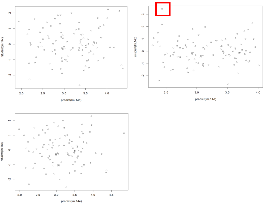
Re-fit the linear models from (c) to (e) using this new data. What effect does this new observation have on the each of the models? In each model, is this observation an outlier? A high-leverage point? Both? Explain your answers.
In the refitting model 14c, the coefficient of x2 becomes statistically significant at the level of 0.01 (β2=2.5146, p-value=0.00614), while the coefficient of x1 becomes statistically insignificant (β1=0.5394, p-value=0.36458).
In the refitting model 14d and 14e, the coefficients of x1 and x2 are both statistically significant at the level of 0.001, which is consistent with previous regression results.
Outliers: Plot the studentized residuals and we can find that all the observations have studentized residuals between -3 and 3 in (c) and (e), which means no outliers are suggested in the models. In the refitting model (d), a point is far from the value cutoff of 3 and it’s marked in the second plot. But we cannot be sure that this outlier is the new observation. The plots of (c) to (e) are shown below.
High-leverage points:
From the plots and the “max hatvalues” command, we can find that in model (c) and (e), the new observation is a high-leverage point. The plots of (c) to (e) are shown below.
1.	> plot(hatvalues (lm.14c))
2.	> which.max(hatvalues (lm.14c))
3.	101
4.	101
5.	> plot(hatvalues (lm.14d))
6.	> which.max(hatvalues (lm.14d))
7.	27
8.	27
9.	> plot(hatvalues (lm.14e))
10.	> which.max(hatvalues (lm.14e))
11.	101
12.	101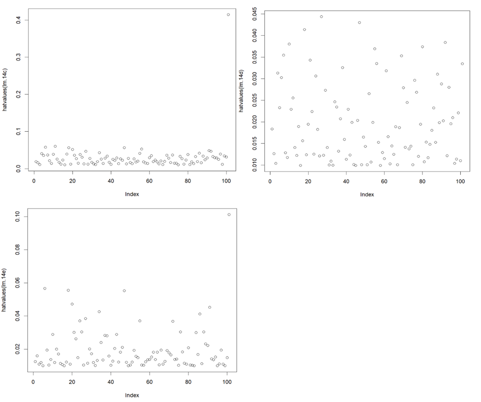


 4539
4539


 被折叠的 条评论
为什么被折叠?
被折叠的 条评论
为什么被折叠?
 到【灌水乐园】发言


