线性回归预测广告投放(一维特征)

载入数据并可视化

# load data
import pandas as pd 
import numpy as np
import matplotlib.pyplot as plt
import seaborn as sns
df_all = pd.read_csv('/kaggle/input/advertising-simple-dataset/advertising.csv')
# virual the data
# 相关性热力图
sns.heatmap(df_all.corr(), cmap='YlGnBu', annot=True)
plt.show()
# visual (scatter plot)
sns.pairplot(df_all,
            x_vars=['wechat', 'weibo', 'others'],
            y_vars='sales',
            height=4, aspect=1, kind='scatter')
plt.show()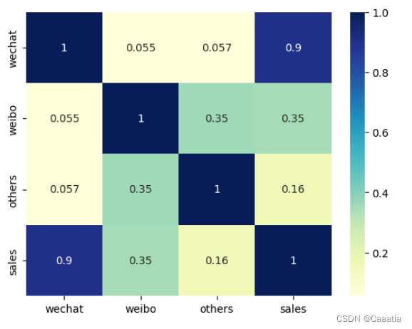

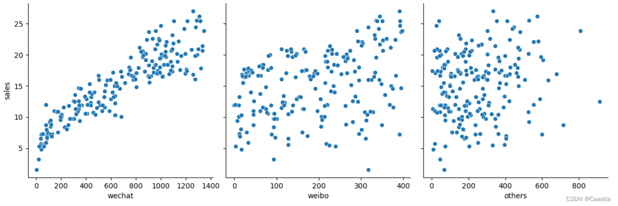
相关性热力图

散点图

明显观测到微信广告投放量与营业额关联度最高，因此先仅考虑wechat这一维度 特征。

数据处理

特征选择

# 因为weibo和others与销售额的相关度不大，所以暂时忽略这两个数据列，构造数据特征和标签
x = np.array(df_all.wechat)
y = np.array(df_all.sales)
# linear regression 模型可接受的输入应该是二维矩阵
# reshape 1D to 2D
x = x.reshape((len(x), 1))
y = y.reshape((len(y), 1))

训练集和测试集拆分

# 训练集和测试集的拆分
from sklearn.model_selection import train_test_split
x_train, x_test, y_train, y_test = train_test_split(x, y, test_size=0.2, random_state=0)

数据归一化

# 数据归一化
# 函数定义
def scaler(train, test):
    min = train.min(axis=0)
    max = train.max(axis=0)
    gap = max - min
    train -= min
    train /= gap
    test -= min
    test /= gap
    return train, test

x_train, x_test = scaler(x_train, x_test)
y_train, y_test = scaler(y_train, y_test)
# 对归一化的数据进行可视化
plt.plot(x_train, y_train, 'r*', label='Training data')
plt.xlabel('wechat')
plt.ylabel('sales')
plt.legend()
plt.show()

模型构建

损失函数

# 定义一个均方差损失函数
def loss_function(x, y, weight, bias):
    y_hat = weight * x + bias
    loss = y_hat - y
    cost = np.sum(loss**2)/(2*len(x))
    return cost

梯度下降

# 自定义梯度下降函数
def gradient_descent(x, y, w, b, lr, iters):
    l_history = np.zeros(iters) # 初始化记录梯度下降cost的数组
    w_history = np.zeros(iters) # 初始化记录历史w的数组
    b_history = np.zeros(iters) # 初始化记录历史b的数组
    for i in range(iters):
        y_hat = x * w + b # 这是假设函数
        loss = y_hat - y # 这是中间过程的loss
        derivative_w = x.T.dot(loss)/len(x) # 对w求导
        derivative_b = sum(loss) * 1/len(x) # 对b求导
        w = w - lr * derivative_w # 更新w
        b = b - lr * derivative_b # 更新b
        l_history[i] = loss_function(x, y, w, b) # 记录第i次循环时候的cost
        w_history[i] = w # 记录第i次循环时候的w
        b_history[i] = b # 记录第i次循环时候的b
    return l_history, w_history, b_history
        
    

模型训练

初始化

# 随机给一个初始的权重和偏置
iterations = 100
alpha = 1
weight = -5
bias = 3
# 计算当前的cost
print("当前的假设函数带来的损失：", loss_function(x_train, y_train, weight, bias))

训练

alpha = 0.8
l_history, w_history, b_history = gradient_descent(x_train, y_train, weight, bias, alpha, iterations)

可视化

# 可视化loss曲线
plt.plot(l_history, 'g--', label = 'loss curve')
plt.xlabel('Iterations')
plt.ylabel('Loss')
plt.legend()
plt.show()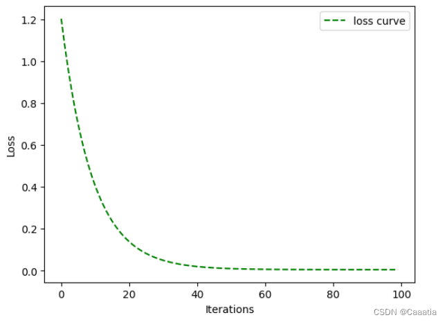

loss图像

print('当前损失：', l_history[-1])
print("当前偏置：", w_history[-1])
print("当前偏置：", b_history[-1])

当前损失： 0.004679247434449546
当前偏置： 0.637595842244559
当前偏置： 0.18593650852725271

# 在测试集上进行预测
print("", loss_function(x_test, y_test, w_history[-1], b_history[-1]))

 0.004751209278505268

相关公式待补全