机器学习之线性回归模型

一、线性回归的一般步骤：

import numpy as np
import matplotlib.pyplot as plt
from sklearn.linear_model import LinearRegression  # 导入包

x = np.linspace(0, 30, 20)  # 创建数据
y = x + 3 * np.random.randn(20)
# print(x)
# print(y)
plt.figure(figsize=(10, 8))
plt.scatter(x, y)  # 绘制初始数据的散点图
plt.show()
model = LinearRegression()  # 初始化一个类
X = x.reshape(-1, 1)  # 将二维数组重整为一个一列的二维数组
Y = y.reshape(-1, 1)
# print(X)
# print(Y)
model.fit(X, Y)
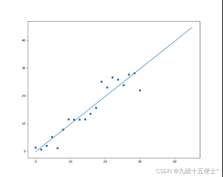
result = model.predict([[40]])  # 预测X=40时的结果
print(result)
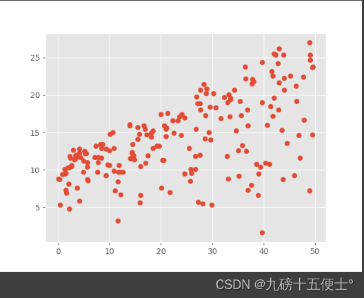
X1 = np.linspace(0, 45).reshape(-1, 1)  # 认为扩大X轴的坐标
plt.figure(figsize=(10, 8))
plt.scatter(X, Y)  # 绘制初始数据的散点图
plt.plot(X1, model.predict(X1))  # 绘制一条线形回归直线
plt.show()

其结果如图所示：

 二、线性回归模型的评价：

# 计算损失值
pridict_result = model.predict(X)  # 计算出所有X对应的预测结果
# print(pridict_result)
sum1 = np.sum(np.square(pridict_result - Y))
print(sum1)  # 预测出模型的损失值
Y_PRE2 = (model.coef_ + 0.1) * X + model.intercept_
# 两个函数分别为模型的斜率和截距
sum2 = np.sum(np.square(Y_PRE2 - Y))
print(sum2)  # 改变预测直线斜率后的损失值
# 可以看出改变斜率过后，损失值明显增大，所以效果比较差

三、客观评价模型的方法

# 客观评价模型的方法
X_train = X[:15]
X_test = X[15:]
Y_train = Y[:15]
Y_test = Y[15:]
model = LinearRegression()
model.fit(X_train, Y_train)
sum3 = np.sum(np.square(model.predict(X_test) - Y_test))
print(sum3)
Y_PRE3 = model.coef_ * X_test + model.intercept_ + 0.5
sum4 = np.sum(np.square(Y_PRE3 - Y_test))
print(sum4)
plt.scatter(X, Y)
plt.plot(X, model.predict(X))
plt.plot(X, model.coef_ * X + model.intercept_ + 0.5)
plt.show()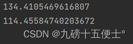

首先可以看出，改变截距之后损失值变小，所以说明预测出来的直线并不是最佳的，这是由于数据的原因。 

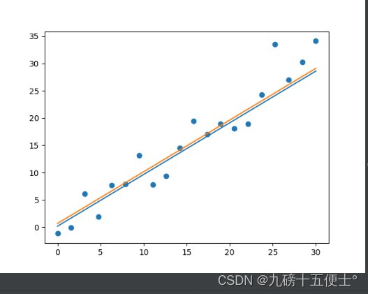
 从图像可以看出，改变截距之后的直线，更能够将所有点平均分在两侧。

四、多元线性回归：

使用广告投放与销售额的数据集，预测销售额与投放量的关系

import numpy as np
import matplotlib.pyplot as plt
from sklearn.linear_model import LinearRegression  # 导入包
from sklearn.model_selection import train_test_split
from sklearn.metrics import mean_squared_error
import pandas as pd
plt.style.use('ggplot')  # 设置绘图样式
data = pd.read_csv('Advertising.csv')
# print(data.head())
plt.scatter(data.TV, data.sales) # 可以看出有明显的线性关系
plt.show()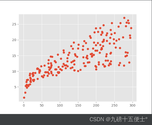

 可以看出TV的投放量与销售额成明显的先行关系

 

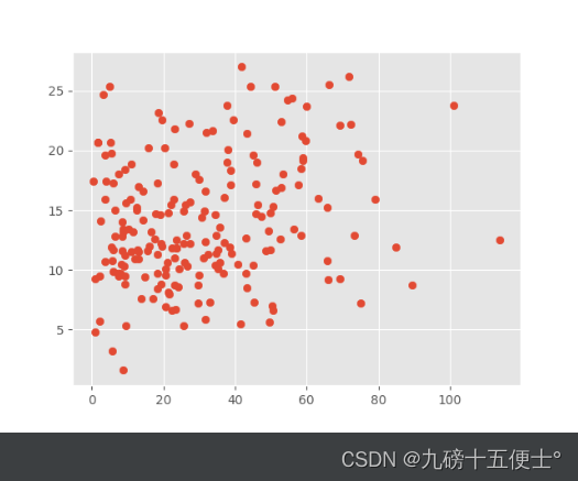
 可以看出radio线性关系较弱，newspaper与销售额都不成线性关系

五、多元回归模型的建立与评价

x = data[['TV', 'radio', 'newspaper']]
y = data.sales
x_train, x_test, y_train, y_test = train_test_split(x, y)  # 将数据集切分为训练集和测试集
model = LinearRegression()
model.fit(x_train, y_train)
# 多远线性回归 y=ax1+bx2+cx3+intc
print(model.coef_)  # 输出a,b,c三个值
print(x_train)
for i in zip(x_train.columns, model.coef_):  # zip()函数用于将两个列表相对应位置的元素打包成元组。
    print(i)
print(mean_squared_error(model.predict(x_test), y_test))  # 用平方差进行验证

 

 看出newspaper的斜率值几乎接近于0，所以影响非常小。

六、多元回归应模型的改进：

将x轴去掉newspaper,再建立模型；

x = data[['TV', 'radio']]
y = data.sales
x_train, x_test, y_train, y_test = train_test_split(x, y)  # 将数据集切分为训练集和测试集
model2 = LinearRegression()
model2.fit(x_train, y_train)
print(model2.coef_)
print(mean_squared_error(model2.predict(x_test), y_test))  # 用平方差进行验证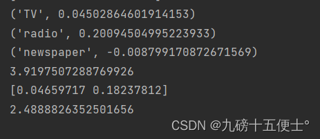

 可以看到平方差验证的值减小了，所以模型比原来的模型更好了，得到了改进。

七、过拟合和欠拟合

过拟合：对训练数据拟合很好，但测试数据表现不好

欠拟合：对训练数据拟合不是很好，测试数据表现也不是很好

首先创建数据集

x = np.linspace(0, 10, 20)
y = x ** 3 + np.random.rand(20) * 160 + 10
plt.scatter(x, y)
plt.show()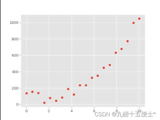

 然后建立模型并绘图：

model = LinearRegression()
model.fit(x.reshape(-1, 1), y)
y_pred = model.predict(x.reshape(-1, 1))
plt.scatter(x, y)
plt.plot(x, y_pred, c='b')
plt.show()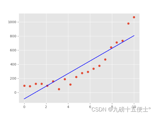

 根据三次方的趋势，可以得出训练数据拟合的不好，未来拟合的效果会更差，所以这就是欠拟合。

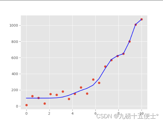
再使用多项式进行拟合，选择4阶多项式

首先导入包

from sklearn.preprocessing import PolynomialFeatures  # 多项式的包

#  使用多项式进行拟合
q4 = PolynomialFeatures(degree=4)
x4 = q4.fit_transform(x.reshape(-1, 1))
model4 = LinearRegression()
model4.fit(x4, y)
y_pred4 = model4.predict(x4)
plt.scatter(x, y)
plt.plot(x, y_pred4, c='b')
plt.show()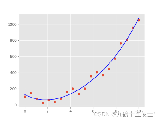

由图可以看出，4阶多项式在训练集中拟合效果很好，如果改为20阶多项式，拟合效果会过分的好。

 

 扩大数据后：

x20 = x[:20]
y20 = y[:20]
print(y20)
q20 = PolynomialFeatures(degree=4)
x20 = q20.fit_transform(x20.reshape(-1, 1))
model4 = LinearRegression()
model4.fit(x20, y20)
y_pred20 = model4.predict(q20.fit_transform(x.reshape(-1, 1)))
plt.scatter(x, y)
plt.plot(x, y_pred20, c='b')
plt.show()

 

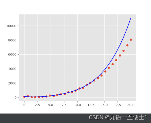
可以看出在训练集中拟合效果很好，到后面的测试集时拟合效果就变的不好，这样的情况就是过拟合。