R语言实现PSM（倾向性评分）（MatchIt包）（1）

weixin_49320263

已于 2023-10-05 19:41:13 修改

阅读量6.8k

点赞数 8

分类专栏：常用方法文章标签： r语言

于 2023-04-07 18:00:17 首次发布

常用方法专栏收录该内容

25 篇文章

订阅专栏

PSM：减少研究中的偏差和混杂变量影响。局限性：条件独立假设，理论上不存在遗漏变量；共同支撑假设，处理组和对照组的倾向得分有较大的共同取值范围，否则不适合做PSM评分。

三个关键：结局指标，目标人群，协变量

R包matchit：初始评估-匹配-结果评估-尝试不同方法-对比不同的匹配情况

（1）导入数据：数据集lalonde中treat为治疗因素，其余变量为协变量。

#PSM
library("MatchIt")
data("lalonde")
head(lalonde)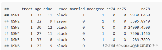

（2）glm：实现广义线性模型；默认为logistics回归

m.out0 <- matchit(treat ~ age + educ + race + married + 
                   nodegree + re74 + re75, data = lalonde,
                 method = NULL, distance = "glm")
# 在匹配前检查平衡
summary(m.out0)

## 
## Call:
## matchit(formula = treat ~ age + educ + race + married + nodegree + 
##     re74 + re75, data = lalonde, method = NULL, distance = "glm")
## 
## Summary of Balance for All Data:
##            Means Treated Means Control Std. Mean Diff. Var. Ratio eCDF Mean eCDF Max
## distance          0.5774        0.1822          1.7941     0.9211    0.3774   0.6444
## age              25.8162       28.0303         -0.3094     0.4400    0.0813   0.1577
## educ             10.3459       10.2354          0.0550     0.4959    0.0347   0.1114
## raceblack         0.8432        0.2028          1.7615          .    0.6404   0.6404
## racehispan        0.0595        0.1422         -0.3498          .    0.0827   0.0827
## racewhite         0.0973        0.6550         -1.8819          .    0.5577   0.5577
## married           0.1892        0.5128         -0.8263          .    0.3236   0.3236
## nodegree          0.7081        0.5967          0.2450          .    0.1114   0.1114
## re74           2095.5737     5619.2365         -0.7211     0.5181    0.2248   0.4470
## re75           1532.0553     2466.4844         -0.2903     0.9563    0.1342   0.2876
## 
## Sample Sizes:
##           Control Treated
## All           429     185
## Matched       429     185
## Unmatched       0       0
## Discarded       0       0

观察Std.Mean Diff.接近于0、Var.Ratio接近于1、eCDF Mean 接近于0、eCDF Max接近于0，表明平衡性良好。

（3）匹配：使用最近邻匹配

# 这次指定method = "nearest"为了实现最近邻匹配，再次使用logistic回归倾向得分。
m.out1 <- matchit(treat ~ age + educ + race + married + 
                   nodegree + re74 + re75, data = lalonde,
                 method = "nearest", distance = "glm")
m.out1

## A matchit object
##  - method: 1:1 nearest neighbor matching without replacement
##  - distance: Propensity score
##              - estimated with logistic regression
##  - number of obs.: 614 (original), 370 (matched)
##  - target estimand: ATT
##  - covariates: age, educ, race, married, nodegree, re74, re75

3、质量评估

#检查匹配后的平衡
summary(m.out1, un = FALSE)
## 
## Call:
## matchit(formula = treat ~ age + educ + race + married + nodegree + 
##     re74 + re75, data = lalonde, method = "nearest", distance = "glm")
## 
## Summary of Balance for Matched Data:
##            Means Treated Means Control Std. Mean Diff. Var. Ratio eCDF Mean eCDF Max Std. Pair Dist.
## distance          0.5774        0.3629          0.9739     0.7566    0.1321   0.4216          0.9740
## age              25.8162       25.3027          0.0718     0.4568    0.0847   0.2541          1.3938
## educ             10.3459       10.6054         -0.1290     0.5721    0.0239   0.0757          1.2474
## raceblack         0.8432        0.4703          1.0259          .    0.3730   0.3730          1.0259
## racehispan        0.0595        0.2162         -0.6629          .    0.1568   0.1568          1.0743
## racewhite         0.0973        0.3135         -0.7296          .    0.2162   0.2162          0.8390
## married           0.1892        0.2108         -0.0552          .    0.0216   0.0216          0.8281
## nodegree          0.7081        0.6378          0.1546          .    0.0703   0.0703          1.0106
## re74           2095.5737     2342.1076         -0.0505     1.3289    0.0469   0.2757          0.7965
## re75           1532.0553     1614.7451         -0.0257     1.4956    0.0452   0.2054          0.7381
## 
## Sample Sizes:
##           Control Treated
## All           429     185
## Matched       185     185
## Unmatched     244       0
## Discarded       0       0
plot(m.out1, type = "jitter", interactive = FALSE)
plot(m.out1, type = "density", interactive = FALSE,
     which.xs = ~age + married + re75)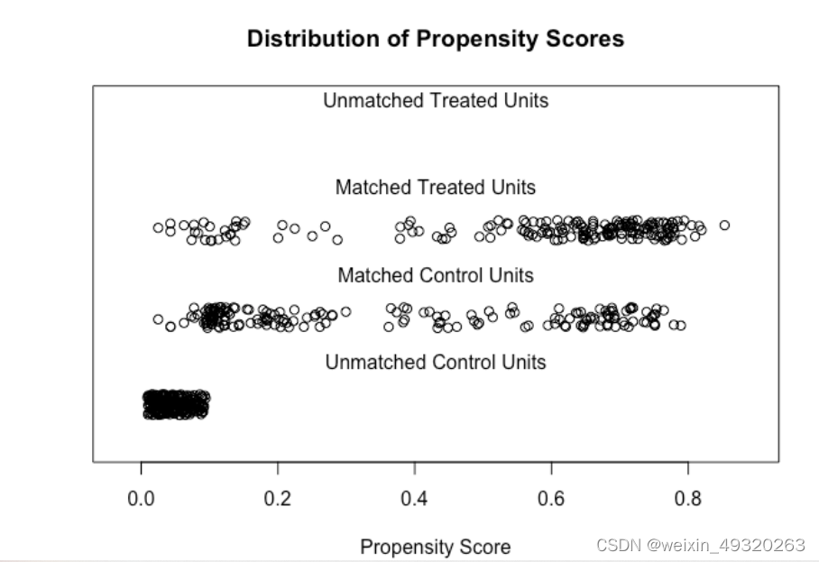

有所改善，但是仍较差， Std. Pair Diff，显示每个协变量的平均绝对值和内部差异。当这些值较小时，通常可以实现更好的平衡。

4、尝试新的匹配方法

# Full matching on a probit PS
m.out2 <- matchit(treat ~ age + educ + race + married + 
                   nodegree + re74 + re75, data = lalonde,
                 method = "full", distance = "glm", link = "probit")
m.out2
## A matchit object
##  - method: Optimal full matching
##  - distance: Propensity score
##              - estimated with probit regression
##  - number of obs.: 614 (original), 614 (matched)
##  - target estimand: ATT
##  - covariates: age, educ, race, married, nodegree, re74, re75
# Checking balance after full matching
summary(m.out2, un = FALSE)
## 
## Call:
## matchit(formula = treat ~ age + educ + race + married + nodegree + 
##     re74 + re75, data = lalonde, method = "full", distance = "glm", 
##     link = "probit")
## 
## Summary of Balance for Matched Data:
##            Means Treated Means Control Std. Mean Diff. Var. Ratio eCDF Mean eCDF Max Std. Pair Dist.
## distance          0.5773        0.5766          0.0036     0.9946    0.0042   0.0541          0.0197
## age              25.8162       25.6335          0.0255     0.4674    0.0819   0.2764          1.2686
## educ             10.3459       10.4590         -0.0562     0.6138    0.0221   0.0595          1.1950
## raceblack         0.8432        0.8389          0.0119          .    0.0043   0.0043          0.0162
## racehispan        0.0595        0.0469          0.0532          .    0.0126   0.0126          0.5068
## racewhite         0.0973        0.1142         -0.0571          .    0.0169   0.0169          0.3978
## married           0.1892        0.1555          0.0860          .    0.0337   0.0337          0.4866
## nodegree          0.7081        0.6711          0.0814          .    0.0370   0.0370          0.9550
## re74           2095.5737     2108.4175         -0.0026     1.3485    0.0330   0.2067          0.8421
## re75           1532.0553     1557.1654         -0.0078     1.5659    0.0509   0.2059          0.8367
## 
## Sample Sizes:
##               Control Treated
## All            429.       185
## Matched (ESS)   51.66     185
## Matched        429.       185
## Unmatched        0.         0
## Discarded        0.         0
plot(summary(m.out2))

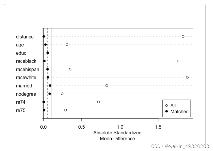
匹配的效果更好。

（6）根据匹配结果进一步分析

m.data <- match.data(m.out2)
head(m.data)
##      treat age educ   race married nodegree re74 re75       re78  distance weights subclass
## NSW1     1  37   11  black       1        1    0    0  9930.0460 0.6356769       1       52
## NSW2     1  22    9 hispan       0        1    0    0  3595.8940 0.2298151       1       61
## NSW3     1  30   12  black       0        0    0    0 24909.4500 0.6813558       1       67
## NSW4     1  27   11  black       0        1    0    0  7506.1460 0.7690590       1       76
## NSW5     1  33    8  black       0        1    0    0   289.7899 0.6954138       1       84
## NSW6     1  22    9  black       0        1    0    0  4056.4940 0.6943658       1       90
library("marginaleffects")
fit <- lm(re78 ~ treat * (age + educ + race + married + nodegree + 
             re74 + re75), data = m.data, weights = weights)
avg_comparisons(fit,
                variables = "treat",
                vcov = ~subclass,
                newdata = subset(m.data, treat == 1),
                wts = "weights")
## 
##   Term Contrast Estimate Std. Error   z Pr(>|z|) 2.5 % 97.5 %
##  treat    1 - 0     1912        765 2.5   0.0124   413   3411
## 
## Columns: term, contrast, estimate, std.error, statistic, p.value, conf.low, conf.high