Kaggle竞赛-Two Sigma Connect: Rental Listing Inquiries（XGBoost）

Kaggle竞赛，网址链接：Two Sigma Connect: Rental Listing Inquiries

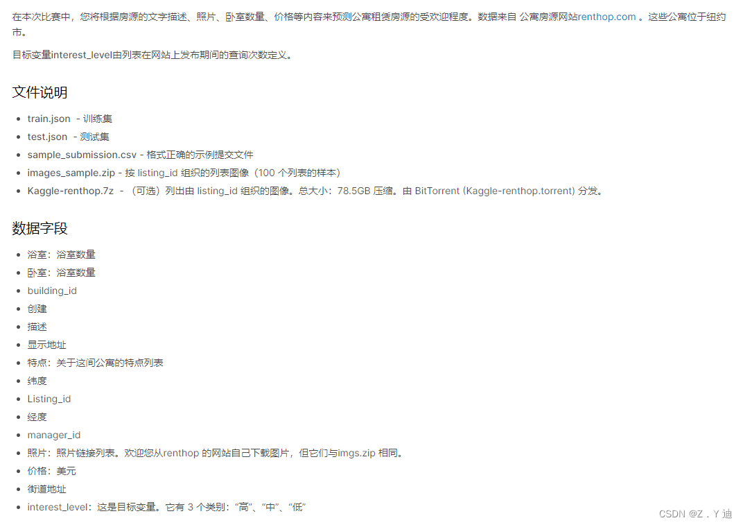
根据租房网站上的数据信息，预测房子的受欢迎程度。（这是一个分类问题，包含以下数据，有类别变量、整数变量、文本变量）。

XGBoost模型

使用sklearn完成建模预测。数据集可在竞赛官网下载。
XGBoost网站
关于XGBoost的讲解，这里不再介绍了。后续，会出一系列的机器学习算法讲解。

import os
import sys
import operator
import numpy as np
import pandas as pd
import zipfile
from scipy import sparse
import xgboost as xgb
from sklearn import model_selection, preprocessing, ensemble
from sklearn.metrics import log_loss
from sklearn.feature_extraction.text import TfidfVectorizer, CountVectorizer

TfidfVectorizer, CountVectorizer查看sklearn官网或者TfidfVectorizer, CountVectorizer

#数据获取，查看另外一篇文章有详细介绍
train_df = pd.read_json(zipfile.ZipFile(r'E:\Kaggle\Kaggle_dataset01\two_sigma\train.json.zip').open('train.json'))
test_df = pd.read_json(zipfile.ZipFile(r'E:\Kaggle\Kaggle_dataset01\two_sigma\test.json.zip').open('test.json'))

另一篇-随机森林方法

#特征工程
features_to_use = ['bathrooms','bedrooms','latitude','longitude','price']
train_df['num_photos'] = train_df['photos'].apply(len)
test_df['num_photos'] = test_df['photos'].apply(len)

train_df['num_features'] = train_df['features'].apply(len)
test_df['num_features'] = test_df['features'].apply(len)

train_df["num_description_words"] = train_df["description"].apply(lambda x: len(x.split(" ")))
test_df["num_description_words"] = test_df["description"].apply(lambda x: len(x.split(" ")))

train_df["created"] = pd.to_datetime(train_df["created"])
test_df["created"] = pd.to_datetime(test_df["created"])

train_df["created_year"] = train_df["created"].dt.year
test_df["created_year"] = test_df["created"].dt.year
train_df["created_month"] = train_df["created"].dt.month
test_df["created_month"] = test_df["created"].dt.month
train_df["created_day"] = train_df["created"].dt.day
test_df["created_day"] = test_df["created"].dt.day
train_df["created_hour"] = train_df["created"].dt.hour
test_df["created_hour"] = test_df["created"].dt.hour

features_to_use.extend(["num_photos", "num_features", "num_description_words","created_year", "created_month", "created_day", "listing_id", "created_hour"])

categorical = ['display_address','manager_id','building_id','street_address']
for f in categorical:
    if train_df[f].dtype == 'object':
        lbl = preprocessing.LabelEncoder()
        lbl.fit(list(train_df[f].values) + list(test_df[f].values))
        train_df[f] = lbl.transform(list(train_df[f].values))
        test_df[f] = lbl.transform(list(test_df[f].values))
        features_to_use.append(f)

train_df['features'] = train_df["features"].apply(lambda x: " ".join(["_".join(i.split(" ")) for i in x]))
test_df['features'] = test_df["features"].apply(lambda x: " ".join(["_".join(i.split(" ")) for i in x]))
print(train_df["features"].head())
tfidf = CountVectorizer(stop_words='english', max_features=200)
tr_sparse = tfidf.fit_transform(train_df["features"])
te_sparse = tfidf.transform(test_df["features"])

train_X = sparse.hstack([train_df[features_to_use], tr_sparse]).tocsr()
test_X = sparse.hstack([test_df[features_to_use], te_sparse]).tocsr()

target_num_map = {'high':0, 'medium':1, 'low':2}
train_y = np.array(train_df['interest_level'].apply(lambda x: target_num_map[x]))
print(train_X.shape, test_X.shape)

#模型搭建
def runXGB(train_X,train_y,test_X,test_y=None,feature_names=None,seed_val=0,num_rounds=1000):
    param = {}
    param['objective'] = 'multi:softprob'
    param['eta'] = 0.1
    param['max_depth'] = 6
    param['silent'] = 1
    param['num_class'] = 3
    param['eval_metric'] = "mlogloss"
    param['min_child_weight'] = 1
    param['subsample'] = 0.7
    param['colsample_bytree'] = 0.7
    param['seed'] = seed_val
    num_rounds = num_rounds
    
    plst = list(param.items())
    
    xgbtrain = xgb.DMatrix(train_X,label=train_y)
    
    if test_y is not None:
        xgbtest = xgb.DMatrix(test_X,label=test_y)
        watchlist = [(xgbtrain,'train'),(xgbtest,'test')]
        model =xgb.train(plst,xgbtrain,num_rounds,watchlist,early_stopping_rounds=20,evals_result=evals_result)
    else:
        xgbtest = xgb.DMatrix(test_X)
        model = xgb.train(plst,xgbtrain,num_rounds)
    pred_test_y = model.predict(xgbtest)
    return pred_test_y,model

#模型训练
cv_scores = []
test_loss = []
train_loss = []
evals_result = {}
import matplotlib.pyplot as plt
kf = model_selection.KFold(n_splits=5,shuffle=True,random_state=12)
for dev_index,val_index in kf.split(range(train_X.shape[0])):
    dev_X, val_X = train_X[dev_index,:], train_X[val_index,:]
    dev_y, val_y = train_y[dev_index], train_y[val_index]
    preds, model = runXGB(dev_X, dev_y, val_X, val_y)
    cv_scores.append(log_loss(val_y, preds))
    print(cv_scores)
    break  #可去掉，将KFlold的所有情况训练一遍。选最好的

#模型训练预测
preds, model = runXGB(train_X, train_y, test_X, num_rounds=400)
out_df = pd.DataFrame(preds)
out_df.columns = ["high", "medium", "low"]
out_df["listing_id"] = test_df.listing_id.values
out_df.to_csv("xgb.csv", index=False)

#模型训练过程分析（loss变化趋势）
import matplotlib.pyplot as plt
plt.figure(figsize=(8,4))
plt.plot(list(range(int(len(evals_result['train']['mlogloss'])))),evals_result['train']['mlogloss'],'r-',label='train_loss')
plt.plot(list(range(int(len(evals_result['test']['mlogloss'])))),evals_result['test']['mlogloss'],'b-',label='test_loss')
plt.legend(loc='upper right')
plt.show()
#如下图

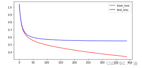
运行上述代码，XGBoost的效果比随机森林好很多，但是还能继续提高。更进一步改进特征工程部分，获取更好的特征（或者使用更好的方法）！