1、Denoising Diffusion Probabilistic Models（扩散模型）

简介

主页：https://hojonathanho.github.io/diffusion/

扩散模型 （diffusion models）是深度生成模型中新的SOTA。

扩散模型在图片生成任务中超越了原SOTA：GAN，并且在诸多应用领域都有出色的表现，如计算机视觉，NLP、波形信号处理、多模态建模、分子图建模、时间序列建模、对抗性净化等。

GAN要训练两个网络，训练难度大，容易不收敛，而且多样性比较差，毕竟生成器是为了骗过鉴别器，生成器可能学到稀奇古怪的技巧，

此外，扩散模型与其他研究领域有着密切的联系，如稳健学习、表示学习、强化学习。

然而，原始的扩散模型也有缺点，它的采样速度慢，通常需要数千个评估步骤才能抽取一个样本；它的最大似然估计无法和基于似然的模型相比；它泛化到各种数据类型的能力较差。

如今很多研究已经从实际应用的角度解决上述限制做出了许多努力，或从理论角度对模型能力进行了分析。但是，现在仍缺乏对扩散模型从算法到应用的最新进展的系统回顾。

基础知识

实现流程

生成式建模的一个核心问题是模型的灵活性和可计算性之间的权衡。

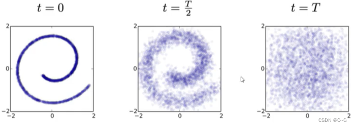
扩散模型的基本思想是正向扩散过程来系统地扰动数据中的分布，然后通过学习反向扩散过程恢复数据的分布，这样就了产生一个高度灵活且易于计算的生成模型。

前向过程

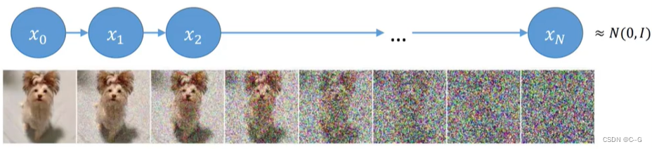
前向过程概括起来就是从原始图像 $X_0$ 开始，不断往图像中加入高斯噪声，每一个时刻由前一时刻的图像增加噪声得到，最后得到纯噪声的图像。这个过程可以看作是不断构建标签（高斯噪声）的过程。

构建 $X_t$ 时刻是公式如下：

$X_t=\sqrt{{\alpha }_t}{X}_{t-1}+\sqrt{1-{\alpha }_t}Z$

其中 ${\alpha }_t=1-{\beta }_t$

$\beta$ 随着时刻 t 增大而增加，论文从0.0001 增加到 0.002。那么 $\alpha$ 随着时刻 t 增大而减少，这表明了后一时刻的图像对前一时刻的图像的依赖逐渐减少，高斯噪声的权重逐渐增大，最后得到纯噪声的图像

从 $X_0$ 开始往后迭代可以得到每一时刻的分布，但是这个过程过于繁琐且消耗大量计算资源，可不可以根据 $X_0$ 获取任意指定时刻的分布呢？

1. 步骤一

   首先，时刻 t 的图像记为 $X_t$，前一时刻 t-1 的图像记为 $X_{t-1}$，这里使用 Z 表示高斯分布

   已知，$X_t=\sqrt{{\alpha }_t}{X}_{t-1}+\sqrt{1-{\alpha }_t}Z$

   将 $X_{t-1}=\sqrt{{\alpha }_{t-1}}{X}_{t-2}+\sqrt{1-{\alpha }_{t-1}}Z$ 代入上述公式，取代 $X_{t-1}$，得到

   $X_t=\sqrt{{\alpha }_t}(\sqrt{{\alpha }_{t-1}}{X}_{t-2}+\sqrt{1-{\alpha }_{t-1}}Z)+\sqrt{1-{\alpha }_t}Z$

   化简得

   $X_t=\sqrt{{\alpha }_t{\alpha }_{t-1}}{X}_{t-2}+\sqrt{{\alpha }_t-{\alpha }_t{\alpha }_{t-1}}Z+\sqrt{1-{\alpha }_t}Z$

2. 步骤二

   高斯分布 $Z\sim \mathrm{N}(0,I)$

   $\sqrt{{\alpha }_t-{\alpha }_t{\alpha }_{t-1}}Z\sim \mathrm{N}(0,{\alpha }_t-{\alpha }_t{\alpha }_{t-1})$

   $\sqrt{1-{\alpha }_t}Z\sim \mathrm{N}(0,1-{\alpha }_t)$

   由于高斯分布符合以下规律

   $\mathrm{N}(0,{\sigma }_1^{2}I)+\mathrm{N}(0,{\sigma }_2^{2}I)\sim \mathrm{N}(0,({\sigma }_1^2+{\sigma }_2^2)I)$

   所以

   $\sqrt{{\alpha }_t-{\alpha }_t{\alpha }_{t-1}}Z+\sqrt{1-{\alpha }_t}Z\sim \mathrm{N}(0,1-{\alpha }_t{\alpha }_{t-1})$

   从步骤一得到的公式：

   $X_t=\sqrt{{\alpha }_t{\alpha }_{t-1}}{X}_{t-2}+\sqrt{{\alpha }_t-{\alpha }_t{\alpha }_{t-1}}Z+\sqrt{1-{\alpha }_t}Z$

   化简可得

   $X_t=\sqrt{{\alpha }_t{\alpha }_{t-1}}{X}_{t-2}+\sqrt{1-{\alpha }_t{\alpha }_{t-1}}Z$

   从而可以推出

   $X_t=\sqrt{\bar{\alpha }}{X}_0+\sqrt{1-\bar{\alpha }}Z$，（$\bar{\alpha }$ 表示连乘）

我们现在可以实现加噪声的过程了，但是目的是去噪生成，也就是接下来的逆向过程

逆向过程

那么我们回到我们的初始目的，如何从 $T_N$ 时刻分布 $X_t$ 一步一步往前推得到生成目标图像 $X_0$ 呢？

回到原始公式

$X_t=\sqrt{{\alpha }_t}{X}_{t-1}+\sqrt{1-{\alpha }_t}Z$

那么我们要如何使用 $X_t$ 表示 $X_{t-1}$呢

1. 步骤一

   这里使用贝叶斯公式

   $q(X_{t-1}|X_t)=q(X_t|X_{t-1})\frac{q(X_{t-1})}{q(X_t)}$

   在前向过程，任意时刻 t 的分布 $X_t$ 可以由 $X_0$ 表示

   $X_t=\sqrt{\bar{\alpha }}{X}_0+\sqrt{1-\bar{\alpha }}Z$，（$\bar{\alpha }$ 表示连乘）

   那么套用贝叶斯的原始公式可以使用初始条件 $X_0$ 表示

   $q(X_{t-1}|X_t,X_0)=q(X_t|X_{t-1},X_0)\frac{q(X_{t-1}|X_0)}{q(X_t|X_0)}$

   右边三项未知数可以表示为：

   $q(X_{t-1}|X_0):\sqrt{{\bar{\alpha }}_{t-1}}{X}_0+\sqrt{1-{\bar{\alpha }}_{t-1}}Z\sim \mathrm{N}(\sqrt{{\bar{\alpha }}_{t-1}}{X}_0,1-{\bar{\alpha }}_{t-1})$

   $q(X_t|X_0):\sqrt{{\bar{\alpha }}_t}{X}_0+\sqrt{1-{\bar{\alpha }}_t}Z\sim \mathrm{N}(\sqrt{{\bar{\alpha }}_t}{X}_0,1-{\bar{\alpha }}_t)$

   $q(X_t|X_{t-1},X_0):\sqrt{{\alpha }_t}{X}_{t-1}+\sqrt{1-{\alpha }_t}Z\sim \mathrm{N}(\sqrt{{\alpha }_t}{X}_{t-1},1-{\alpha }_t)$

   将上面三条公式带入贝叶斯公式

   $q(X_{t-1}|X_t,X_0)=q(X_t|X_{t-1},X_0)\frac{q(X_{t-1}|X_0)}{q(X_t|X_0)}$

   我们知道高斯分布 $Z=e^{-\frac{1}{2}\frac{(x-\mu {)}^2}{{\sigma }^2}}$

   化简得到

   $X_{t-1}=e^{(-\frac{1}{2}(\frac{(x_t-\sqrt{{\alpha }_t}{X}_{t-1}{)}^2}{{\beta }_t}+\frac{(X_{t-1}-\sqrt{{\bar{\alpha }}_{t-1}}{X}_0{)}^2}{1-{\bar{\alpha }}_{t-1}}-\frac{(X_t-\sqrt{{\bar{\alpha }}_t}{X}_0{)}^2}{1-{\bar{\alpha }}_t}))}$

2. 步骤二

   将步骤一的 $X_{t-1}$ 表达式展开后，汇总化简得到

   $e^{(-\frac{1}{2}((\frac{{\alpha }_t}{{\beta }_t}+\frac{1}{1-{\bar{\alpha }}_{t-1}})X_{t-1}^2-(\frac{2\sqrt{{\alpha }_t}}{{\beta }_t}{X}_t+\frac{2\sqrt{{\bar{\alpha }}_{t-1}}}{1-{\bar{\alpha }}_{t-1}}{X}_0)X_{t-1}+C(X_t,X_0)))}$

   $C(X_t,X_0)$ 为常数项，不影响任务，核心是求 $X_t$ 与 $X_{t-1}$ 的关系。

   将高斯分布(Z) 展开后为

   $Z=e^{(-\frac{(x-\mu {)}^2}{2{\sigma }^2})}=e^{(-\frac{1}{2}(\frac{1}{{\sigma }^2}{X}^2-\frac{2\mu }{{\sigma }^2}X+\frac{{\mu }^2}{{\sigma }^2}))}$

   对比 高斯分布(Z) 展开后公式 与 上述得到的 $X_{t-1}$ 表达式，可以得到 均值 和 方差
   $\frac{1}{{\sigma }^2}=(\frac{{\alpha }_t}{{\beta }_t}+\frac{1}{1-{\bar{\alpha }}_{t-1}})$

   $\sigma =\frac{1-{\bar{\alpha }}_{t-1}}{1-{\bar{\alpha }}_t}{\beta }_t$

   $\tilde{\mu }(X_t,X_0)=\frac{{\sqrt{\alpha }}_t(1-{\bar{\alpha }}_{t-1})}{1-{\bar{\alpha }}_t}{X}_t+\frac{\sqrt{{\bar{\alpha }}_{t-1}}{\beta }_t}{1-{\bar{\alpha }}_t}{X}_0$

   其中 $X_0$ 未知，但是我们知道 $X_t$ 可以由 $X_0$ 得到，那么将原公式逆过来

   $X_t=\sqrt{\bar{\alpha }}{X}_0+\sqrt{1-\bar{\alpha }}Z$，（$\bar{\alpha }$ 表示连乘）

   $X_0=\frac{1}{\sqrt{{\bar{\alpha }}_t}}(X_t-\sqrt{1-{\bar{\alpha }}_t}Z)$

   再将 $X_0$ 带入均值表达式，化简得

   ${\tilde{\mu }}_t=\frac{1}{\sqrt{{\alpha }_t}}(X_t-\frac{{\beta }_t}{\sqrt{1-{\bar{\alpha }}_t}}Z)$

3. 步骤三

   每一时刻的 $X_t$ 都是一个高斯分布，因此，可以通过高斯分布重采样策略得到 $X_{t-1}$

   我们现在得到了有样本 X 得到的分布 $X\sim N(\mu ,{\sigma }^2)$。采样这个操作本身是不可导的，但是我们可以通过重参数化技巧，将简单分布的采样结果变换到特定分布中，如此一来则可以对变换过程进行求导。具体而言，我们从标准高斯分布中采样，并将其变换到$X\sim N(\mu ,{\sigma }^2)$，过程如下

   $\epsilon \sim \mathrm{N}(0,I)$
   $Z=\mu +\sigma \times \epsilon$

   也就是说，从 $\mathrm{N}(\mu ,{\sigma }^2)$ 采样 $Z$，等同于从 $\epsilon \sim \mathrm{N}(0,I)$ 中采样高斯噪声 $\epsilon$，再将其按 $Z=\mu +\sigma \times \epsilon$ 变换

   $X_{t-1}={\tilde{\mu }}_t+{\sigma }_{t}Z\sim \mathrm{N}({\tilde{\mu }}_t,{\sigma }_t)$

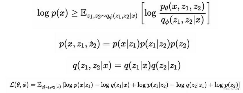
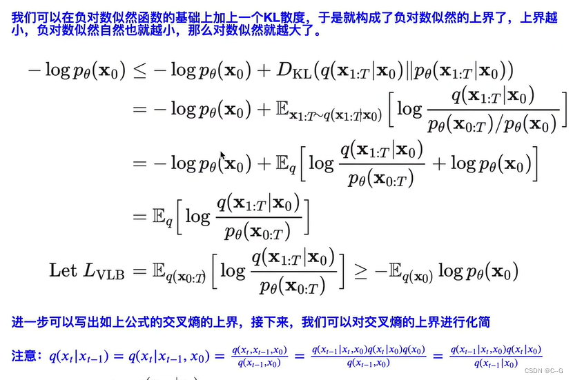
目标数据分布的似然函数

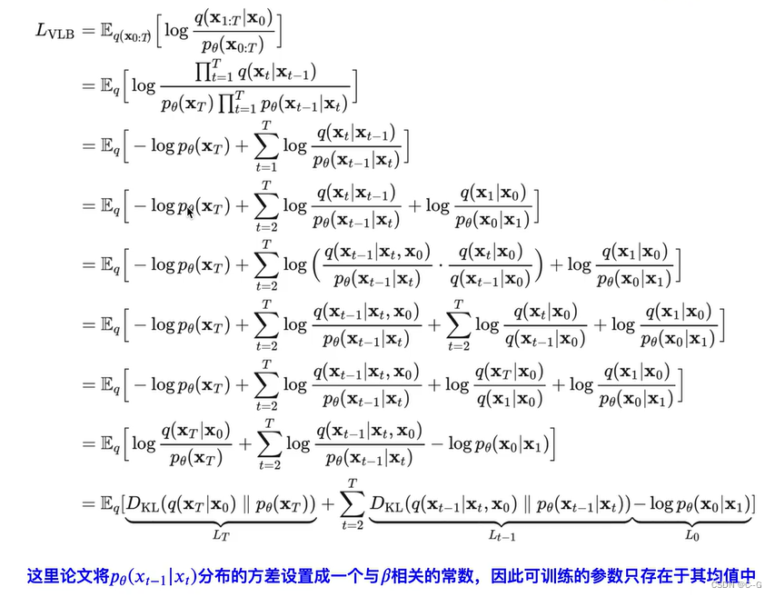
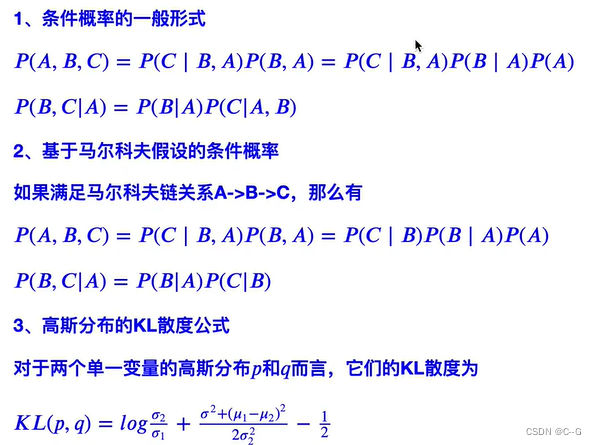
对于两个单一变量的高斯分布 p 和 q而言，KL散度为$KL(p,q)=\log \frac{{\sigma }_2}{{\sigma }_1}+\frac{{\sigma }_1^2+({\mu }_1-{\mu }_2{)}^2}{2{\sigma }_2^2}-\frac{1}{2}$

伪代码

总体网络可以采用了简单的U-net实现

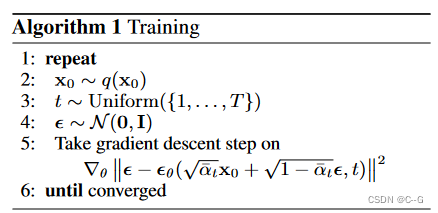
Training

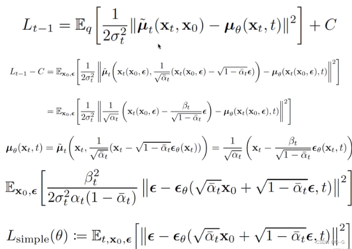
目标：让网络预测不同时刻的高斯分布 ${\epsilon }_{\theta }$

首先从数据集中随机采样图像 $X_0$，选取超参数时刻上限 $T$，在$1,...,T$ 中随机采样时刻（batch size）并为此生成时刻对应的高斯分布 $\epsilon$，根据公式

$X_t=\sqrt{\bar{\alpha }}{X}_0+\sqrt{1-\bar{\alpha }}Z$，（$\bar{\alpha }$ 表示连乘）

将 t 时刻的分布 $X_t$ 和时刻 t 输入网络，其中时刻 t 经过位置编码后与 $X_t$ 拼接，网络预测得到时刻 t 的高斯分布 ${\epsilon }_{\theta }$，将其与对应时刻的高斯分布 $\epsilon$ 作 $L_2$ 损失

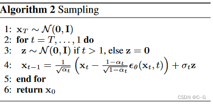
Sampling

分布 $X_t$ 由高斯分布给出，进行 $T$ 次循环，从模型${\epsilon }_{\theta }(X_t,t)$中获取时刻 t 的高斯分布预测值 ${\epsilon }_{\theta }$，通过公式：

$X_{t-1}={\tilde{\mu }}_t+{\sigma }_{t}Z\sim \mathrm{N}({\tilde{\mu }}_t,{\sigma }_t)$

预测前一时刻的分布 $X_{t-1}$，循环该过程得到最终图像 $X_0$

扩散模型代码

class GaussianDiffusion:
  """
  Contains utilities for the diffusion model.
  """

  def __init__(self, *, betas, loss_type, tf_dtype=tf.float32):
    self.loss_type = loss_type

    assert isinstance(betas, np.ndarray)
    self.np_betas = betas = betas.astype(np.float64)  # computations here in float64 for accuracy
    assert (betas > 0).all() and (betas <= 1).all()
    timesteps, = betas.shape
    self.num_timesteps = int(timesteps)

    alphas = 1. - betas
    alphas_cumprod = np.cumprod(alphas, axis=0)
    alphas_cumprod_prev = np.append(1., alphas_cumprod[:-1])
    assert alphas_cumprod_prev.shape == (timesteps,)

    self.betas = tf.constant(betas, dtype=tf_dtype)
    self.alphas_cumprod = tf.constant(alphas_cumprod, dtype=tf_dtype)
    self.alphas_cumprod_prev = tf.constant(alphas_cumprod_prev, dtype=tf_dtype)

    # calculations for diffusion q(x_t | x_{t-1}) and others
    self.sqrt_alphas_cumprod = tf.constant(np.sqrt(alphas_cumprod), dtype=tf_dtype)
    self.sqrt_one_minus_alphas_cumprod = tf.constant(np.sqrt(1. - alphas_cumprod), dtype=tf_dtype)
    self.log_one_minus_alphas_cumprod = tf.constant(np.log(1. - alphas_cumprod), dtype=tf_dtype)
    self.sqrt_recip_alphas_cumprod = tf.constant(np.sqrt(1. / alphas_cumprod), dtype=tf_dtype)
    self.sqrt_recipm1_alphas_cumprod = tf.constant(np.sqrt(1. / alphas_cumprod - 1), dtype=tf_dtype)

    # -------------- 方差

    # calculations for posterior q(x_{t-1} | x_t, x_0)
    posterior_variance = betas * (1. - alphas_cumprod_prev) / (1. - alphas_cumprod)
    # above: equal to 1. / (1. / (1. - alpha_cumprod_tm1) + alpha_t / beta_t)
    self.posterior_variance = tf.constant(posterior_variance, dtype=tf_dtype)
    # below: log calculation clipped because the posterior variance is 0 at the beginning of the diffusion chain

    # sqrt_alphas  sqrt_0.0001 一开始很小 为了避免为0，取对数
    self.posterior_log_variance_clipped = tf.constant(np.log(np.maximum(posterior_variance, 1e-20)), dtype=tf_dtype)

    # -------------- 均值
    # 知道 X_0 的情况下计算 均值 后部分
    self.posterior_mean_coef1 = tf.constant(
      betas * np.sqrt(alphas_cumprod_prev) / (1. - alphas_cumprod), dtype=tf_dtype)
    # 知道 X_0 的情况下计算 均值 前部分
    self.posterior_mean_coef2 = tf.constant(
      (1. - alphas_cumprod_prev) * np.sqrt(alphas) / (1. - alphas_cumprod), dtype=tf_dtype)

  @staticmethod
  def _extract(a, t, x_shape):
    """
    从 a 中按t抽取元素
    Extract some coefficients at specified timesteps,
    then reshape to [batch_size, 1, 1, 1, 1, ...] for broadcasting purposes.
    """
    bs, = t.shape
    assert x_shape[0] == bs
    out = tf.gather(a, t)
    assert out.shape == [bs]
    return tf.reshape(out, [bs] + ((len(x_shape) - 1) * [1]))

#  ======================= 加噪过程 q(z | x)  =======================

  def q_mean_variance(self, x_start, t):
    """
    加噪过程 计算 X_t 均值和方差
    """
    mean = self._extract(self.sqrt_alphas_cumprod, t, x_start.shape) * x_start
    variance = self._extract(1. - self.alphas_cumprod, t, x_start.shape)
    log_variance = self._extract(self.log_one_minus_alphas_cumprod, t, x_start.shape)
    return mean, variance, log_variance

  def q_sample(self, x_start, t, noise=None):
    """
    Diffuse the data (t == 0 means diffused for 1 step)
    根据 X_0,t 计算 X_t 时刻分布
    """
    if noise is None:
      noise = tf.random_normal(shape=x_start.shape)
    assert noise.shape == x_start.shape
    return (
        self._extract(self.sqrt_alphas_cumprod, t, x_start.shape) * x_start +
        self._extract(self.sqrt_one_minus_alphas_cumprod, t, x_start.shape) * noise
    )


#  ======================= 模型损失、验证  =======================


  def p_losses(self, denoise_fn, x_start, t, noise=None):
    """
    Training loss calculation
    训练过程，模型 预测噪声 与 标注正态分布
    """
    B, H, W, C = x_start.shape.as_list()
    assert t.shape == [B]

    if noise is None:
      noise = tf.random_normal(shape=x_start.shape, dtype=x_start.dtype)
    assert noise.shape == x_start.shape and noise.dtype == x_start.dtype
    x_noisy = self.q_sample(x_start=x_start, t=t, noise=noise)
    x_recon = denoise_fn(x_noisy, t)
    assert x_noisy.shape == x_start.shape
    assert x_recon.shape[:3] == [B, H, W] and len(x_recon.shape) == 4

    if self.loss_type == 'noisepred':
      # predict the noise instead of x_start. seems to be weighted naturally like SNR
      assert x_recon.shape == x_start.shape
      losses = nn.meanflat(tf.squared_difference(noise, x_recon))
    else:
      raise NotImplementedError(self.loss_type)

    assert losses.shape == [B]
    return losses

#  ======================= 去噪过程 p(z | x)  =======================

  def q_posterior(self, x_start, x_t, t):
    """
    Compute the mean and variance of the diffusion posterior q(x_{t-1} | x_t, x_0)
    根据 x_0 x_t t 计算方差 和 均值
    """
    assert x_start.shape == x_t.shape
    posterior_mean = (
        self._extract(self.posterior_mean_coef1, t, x_t.shape) * x_start +
        self._extract(self.posterior_mean_coef2, t, x_t.shape) * x_t
    )
    posterior_variance = self._extract(self.posterior_variance, t, x_t.shape)
    posterior_log_variance_clipped = self._extract(self.posterior_log_variance_clipped, t, x_t.shape)
    assert (posterior_mean.shape[0] == posterior_variance.shape[0] == posterior_log_variance_clipped.shape[0] ==
            x_start.shape[0])
    return posterior_mean, posterior_variance, posterior_log_variance_clipped

  def predict_start_from_noise(self, x_t, t, noise):
    """
    根据 X_t t 计算 X_0
    """
    assert x_t.shape == noise.shape
    return (
        self._extract(self.sqrt_recip_alphas_cumprod, t, x_t.shape) * x_t -
        self._extract(self.sqrt_recipm1_alphas_cumprod, t, x_t.shape) * noise
    )

  def p_mean_variance(self, denoise_fn, *, x, t, clip_denoised: bool):
    """
      去噪过程获取 均值 和 方差
    """
    if self.loss_type == 'noisepred':
      x_recon = self.predict_start_from_noise(x, t=t, noise=denoise_fn(x, t))
    else:
      raise NotImplementedError(self.loss_type)

    if clip_denoised:
      x_recon = tf.clip_by_value(x_recon, -1., 1.)

    model_mean, posterior_variance, posterior_log_variance = self.q_posterior(x_start=x_recon, x_t=x, t=t)
    assert model_mean.shape == x_recon.shape == x.shape
    assert posterior_variance.shape == posterior_log_variance.shape == [x.shape[0], 1, 1, 1]
    return model_mean, posterior_variance, posterior_log_variance

  def p_sample(self, denoise_fn, *, x, t, noise_fn, clip_denoised=True, repeat_noise=False):
    """
    Sample from the model
    计算 X_t
    """
    model_mean, _, model_log_variance = self.p_mean_variance(denoise_fn, x=x, t=t, clip_denoised=clip_denoised)
    noise = noise_like(x.shape, noise_fn, repeat_noise)
    assert noise.shape == x.shape
    # no noise when t == 0
    nonzero_mask = tf.reshape(1 - tf.cast(tf.equal(t, 0), tf.float32), [x.shape[0]] + [1] * (len(x.shape) - 1))

    # tf.exp(0.5 * model_log_variance) 去掉 log
    return model_mean + nonzero_mask * tf.exp(0.5 * model_log_variance) * noise

  def p_sample_loop(self, denoise_fn, *, shape, noise_fn=tf.random_normal):
    """
    Generate samples
    循环 去噪过程
    """
    i_0 = tf.constant(self.num_timesteps - 1, dtype=tf.int32)
    assert isinstance(shape, (tuple, list))
    img_0 = noise_fn(shape=shape, dtype=tf.float32)
    _, img_final = tf.while_loop(
      cond=lambda i_, _: tf.greater_equal(i_, 0),
      body=lambda i_, img_: [
        i_ - 1,
        self.p_sample(denoise_fn=denoise_fn, x=img_, t=tf.fill([shape[0]], i_), noise_fn=noise_fn)
      ],
      loop_vars=[i_0, img_0],
      shape_invariants=[i_0.shape, img_0.shape],
      back_prop=False
    )
    assert img_final.shape == shape
    return img_final

#  ======================= 验证过程  =======================

  def p_sample_loop_trajectory(self, denoise_fn, *, shape, noise_fn=tf.random_normal, repeat_noise_steps=-1):
    """
    生成样本，返回中间图像用于可视化去噪图像如何随时间演变


    Generate samples, returning intermediate images
    Useful for visualizing how denoised images evolve over time
    Args:
      repeat_noise_steps (int): Number of denoising timesteps in which the same noise
        is used across the batch. If >= 0, the initial noise is the same for all batch elemements.
    """
    i_0 = tf.constant(self.num_timesteps - 1, dtype=tf.int32)
    assert isinstance(shape, (tuple, list))
    img_0 = noise_like(shape, noise_fn, repeat_noise_steps >= 0)
    times = tf.Variable([i_0])
    imgs = tf.Variable([img_0])

    # 相同噪声的步骤
    # Steps with repeated noise
    times, imgs = tf.while_loop(
      cond=lambda times_, _: tf.less_equal(self.num_timesteps - times_[-1], repeat_noise_steps),
      body=lambda times_, imgs_: [
        tf.concat([times_, [times_[-1] - 1]], 0),
        tf.concat([imgs_, [self.p_sample(denoise_fn=denoise_fn,
                                         x=imgs_[-1],
                                         t=tf.fill([shape[0]], times_[-1]),
                                         noise_fn=noise_fn,
                                         repeat_noise=True)]], 0)
      ],
      loop_vars=[times, imgs],
      shape_invariants=[tf.TensorShape([None, *i_0.shape]),
                        tf.TensorShape([None, *img_0.shape])],
      back_prop=False
    )

    # 每个批处理元素具有不同噪声的步骤
    # Steps with different noise for each batch element
    times, imgs = tf.while_loop(
      cond=lambda times_, _: tf.greater_equal(times_[-1], 0),
      body=lambda times_, imgs_: [
        tf.concat([times_, [times_[-1] - 1]], 0),
        tf.concat([imgs_, [self.p_sample(denoise_fn=denoise_fn,
                                         x=imgs_[-1],
                                         t=tf.fill([shape[0]], times_[-1]),
                                         noise_fn=noise_fn,
                                         repeat_noise=False)]], 0)
      ],
      loop_vars=[times, imgs],
      shape_invariants=[tf.TensorShape([None, *i_0.shape]),
                        tf.TensorShape([None, *img_0.shape])],
      back_prop=False
    )
    assert imgs[-1].shape == shape
    return times, imgs

  def interpolate(self, denoise_fn, *, shape, noise_fn=tf.random_normal):
    """
    在图像之间插入。
    Interpolate between images.
    t == 0 means diffuse images for 1 timestep before mixing.
    """
    assert isinstance(shape, (tuple, list))

    # 占位符，用于插入真实样本
    # Placeholders for real samples to interpolate
    x1 = tf.placeholder(tf.float32, shape)
    x2 = tf.placeholder(tf.float32, shape)
    # lam == 0.5 averages diffused images.
    lam = tf.placeholder(tf.float32, shape=())
    t = tf.placeholder(tf.int32, shape=())

    # 通过前向扩散添加噪声
    # Add noise via forward diffusion
    # TODO: use the same noise for both endpoints?
    # t_batched = tf.constant([t] * x1.shape[0], dtype=tf.int32)
    t_batched = tf.stack([t] * x1.shape[0])
    xt1 = self.q_sample(x1, t=t_batched)
    xt2 = self.q_sample(x2, t=t_batched)

    # Mix latents
    # Linear interpolation
    xt_interp = (1 - lam) * xt1 + lam * xt2
    # Constant variance interpolation
    # xt_interp = tf.sqrt(1 - lam * lam) * xt1 + lam * xt2

    # Reverse diffusion (similar to self.p_sample_loop)
    # t = tf.constant(t, dtype=tf.int32)
    _, x_interp = tf.while_loop(
      cond=lambda i_, _: tf.greater_equal(i_, 0),
      body=lambda i_, img_: [
        i_ - 1,
        self.p_sample(denoise_fn=denoise_fn, x=img_, t=tf.fill([shape[0]], i_), noise_fn=noise_fn)
      ],
      loop_vars=[t, xt_interp],
      shape_invariants=[t.shape, xt_interp.shape],
      back_prop=False
    )
    assert x_interp.shape == shape

    return x1, x2, lam, x_interp, t