


速览:
目录
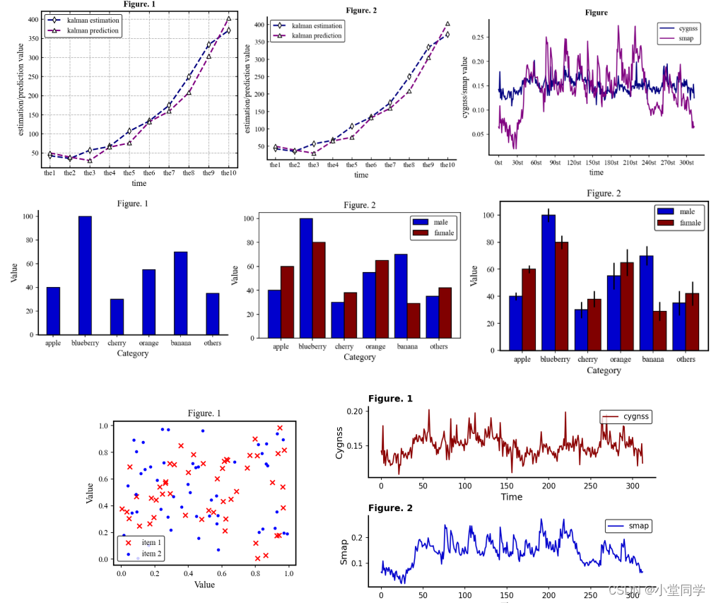
一、线型图
图1、2代码
import matplotlib.pyplot as plt
import numpy as np
plt.rc('font',family='Times New Roman')

estimation = [42.8, 35.6, 57.24, 67.14, 107.19, 133.84, 175.02, 249.91, 333.99, 371.07]
prediction = [50, 39.199999999999996, 30.200000000000003, 65.34, 76.14,
			  131.69, 159.39000000000001, 208.37, 304.01, 403.09000000000003]

# 绘图 #
fig, ax1 = plt.subplots(figsize=(5, 4))
x = np.linspace(0,400,len(estimation))
ax1.axis('auto')	# 参数 'scale','auto','square'
ax1.plot(x, estimation, 'd--', c='navy', linewidth=2, markerfacecolor='w',
		 markeredgecolor='k', label='kalman estimation')
ax1.plot(x, prediction, '^--', c='purple', linewidth=2, markerfacecolor='w',
		 markeredgecolor='k', label='kalman prediction')
ax1.set_xlabel('time', fontsize=12)
ax1.set_ylabel('estimation/prediction value', fontsize=12)
ax1.set_title('Figure. 1',fontweight='bold', fontsize=12)
ax1.set_xticks(x)
ax1.set_xticklabels(['the' + str(i) for i in range(1, 11, 1)])
ax1.tick_params(top=True,right=True,direction='in')		# 右边和上边的刻度都显示,且刻度向内。
ax1.legend(fontsize=10, edgecolor='black')
ax1.spines['bottom'].set_linewidth(1.5)
ax1.spines['left'].set_linewidth(1.5)
ax1.spines['right'].set_linewidth(1.5)
ax1.spines['top'].set_linewidth(1.5)
ax1.grid(axis='both', ls='--')	# axis = 'both','x','y'

fig2, ax2 = plt.subplots(figsize=(5, 4))
x = np.linspace(0,400,len(estimation))
ax2.axis('auto')	# 参数 'scale','auto','square'
ax2.plot(x, estimation, 'd--', c='navy', linewidth=2, markerfacecolor='w',
		 markeredgecolor='k', label='kalman estimation')
ax2.plot(x, prediction, '^--', c='purple', linewidth=2, markerfacecolor='w',
		 markeredgecolor='k', label='kalman prediction')
ax2.set_xlabel('time', fontsize=12)
ax2.set_ylabel('estimation/prediction value', fontsize=12)
ax2.set_title('Figure. 2',fontweight='bold', fontsize=12)
ax2.set_xticks(x)
ax2.set_xticklabels(['the' + str(i) for i in range(1, 11, 1)])
ax2.legend(fontsize=10, edgecolor='black')
ax2.tick_params(direction='in')
ax2.spines['right'].set_visible(False)
ax2.spines['top'].set_visible(False)
ax2.spines['bottom'].set_linewidth(1.5)
ax2.spines['left'].set_linewidth(1.5)
ax2.spines['right'].set_linewidth(1.5)
ax2.spines['top'].set_linewidth(1.5)
# ax2.grid(axis='y', ls='--')	# axis = 'both','x','y'

plt.show()
图3 代码
import numpy as np
import matplotlib.pyplot as plt
import pandas as pd

df = pd.read_excel("时序.xlsx")
time = df["time"]
time_ls = []
for i in range(len(time)):
	temp = str(time[i])
	temp = temp.replace(" 00:00:00", "")
	time_ls.append(str(temp))

cygnss = df['A']
cygnss = np.array(cygnss)
smap = df['B']
smap = np.array(smap)
M = len(smap)
# ========绘图=========== #
plt.rc('font',family='Times New Roman')
fig,ax = plt.subplots(figsize=(6,4))
ax.axis('auto')
ax.plot(cygnss,'-',c='navy',label='cygnss')
ax.plot(smap,'-',c='purple',label='smap')
ax.set_xlabel('time',fontsize=12)
ax.set_ylabel('cygnss/smap value',fontsize=12)
ax.set_title('Figure',fontsize=12,fontweight='bold')
ax.tick_params(direction='in')
ax.legend(fontsize=10,edgecolor='black')
ax.spines['right'].set_visible(False)
ax.spines['top'].set_visible(False)
ax.spines['bottom'].set_linewidth(1.5)
ax.spines['left'].set_linewidth(1.5)
ax.spines['right'].set_linewidth(1.5)
ax.spines['top'].set_linewidth(1.5)
ax.set_xticks(np.arange(0,M,30),[str(i)+'st' for i in np.arange(0,M,30)])
plt.show()
二、条形图
图4,5,6代码(图6 将误差参数去掉即为图5)
import matplotlib.pyplot as plt
import numpy as np
plt.rc('font',family='Times New Roman')

fig, ax = plt.subplots(figsize=(5,4))
ax.axis('auto')
fruits = ['apple', 'blueberry', 'cherry', 'orange','banana','others']
counts = [40, 100, 30, 55, 70, 35]
ax.bar(fruits,counts,width=0.4,edgecolor='black',color='mediumblue')
ax.set_xlabel('Category',fontsize=12)
ax.set_ylabel('Value',fontsize=12)
ax.tick_params(direction='in')
ax.set_title('Figure. 1',fontsize=12,fontweight='bold')
for i in ['bottom','left','right','top']:
	ax.spines[i].set_linewidth(1.5)
ax.spines['right'].set_visible(False)
ax.spines['top'].set_visible(False)


fig2,ax2 = plt.subplots(figsize=(5,4))
ax2.axis('auto')
fruits = ['apple', 'blueberry', 'cherry', 'orange','banana','others']
count1 = [40, 100, 30, 55, 70, 35]
count2 = [60, 80, 38, 65, 29, 42]
x = np.arange(len(count2))
width = 0.4
error = np.array([3,5,6,10,7,9])
for i in ['bottom','left','right','top']:
	ax2.spines[i].set_linewidth(1.5)
ax2.bar(x-width/2,count1,width=width,yerr=error,label='male',color='mediumblue',edgecolor='black')
ax2.bar(x+width/2,count2,width=width,yerr=error,label='famale',color='maroon',edgecolor='black')
ax2.legend(fontsize=10,edgecolor='black')
ax2.set_xticks(x,fruits)
ax2.set_xlabel('Category',fontsize=12)
ax2.tick_params(top=True,right=True,direction='in')
ax2.set_ylabel('Value',fontsize=12)
ax2.set_title('Figure. 2',fontsize=12,fontweight='bold')
plt.show()
三、散点图
图7 代码
import matplotlib.pyplot as plt
import numpy as np
x = np.random.rand(50,1)
y = np.random.rand(50,1)

plt.rc('font',family='Times New Roman')

fig,ax = plt.subplots(figsize=(5,4))
for i in ['bottom','left','right','top']:
	ax.spines[i].set_linewidth(1.5)
ax.scatter(x,y,marker='x',color='r',label='item 1')

a = np.random.rand(50,1)
b = np.random.rand(50,1)
ax.scatter(a,b,marker='.',color='b',label='item 2')
ax.set_xlabel('Value',fontsize=12)
ax.set_ylabel('Value',fontsize=12)
ax.tick_params(right=True,top=True,direction='in')
ax.set_title('Figure. 1',fontsize=12)
ax.legend(loc='best',fontsize=10,edgecolor='black')
plt.show()
四、子图
图8 代码
import numpy as np
import matplotlib.pyplot as plt
import pandas as pd
plt.rc('font',family='Times New Roman')

df = pd.read_excel("时序.xlsx")
time = df["time"]
time_ls = []
for i in range(len(time)):
	temp = str(time[i])
	temp = temp.replace(" 00:00:00", "")
	time_ls.append(str(temp))

cygnss = df['A']
cygnss = np.array(cygnss)
smap = df['B']
smap = np.array(smap)
M = len(smap)

fig,[ax1,ax2] = plt.subplots(2,1,figsize=(8,5))

ax1.axis('auto')
ax1.plot(cygnss,'-',color='darkred',label='cygnss',)
ax1.spines['right'].set_visible(False)
ax1.spines['top'].set_visible(False)
ax1.set_ylabel('Cygnss',fontsize=12)
ax1.legend(fontsize=10,edgecolor='black',loc='upper right')
ax1.set_title('Figure. 1',fontweight='bold',loc='left')
ax1.set_xlabel('Time',fontsize=12)

for i in ['bottom','left','right','top']:
	ax1.spines[i].set_linewidth(1.5)
	ax2.spines[i].set_linewidth(1.5)

ax2.plot(smap,label='smap',color='mediumblue')
ax2.spines['right'].set_visible(False)
ax2.spines['top'].set_visible(False)
ax2.set_ylabel('Smap',fontsize=12)
ax2.set_xlabel('Time',fontsize=12)
ax2.legend(fontsize=10,edgecolor='black',loc='upper right')
ax2.set_title('Figure. 2',fontweight='bold',loc='left')

fig.tight_layout()  # 紧凑布局
plt.show()


 3506
3506


 被折叠的 条评论
为什么被折叠?
被折叠的 条评论
为什么被折叠?
 到【灌水乐园】发言


