【机器学习】Model Evaluation 常用模型评估方法 + Python代码实现

---

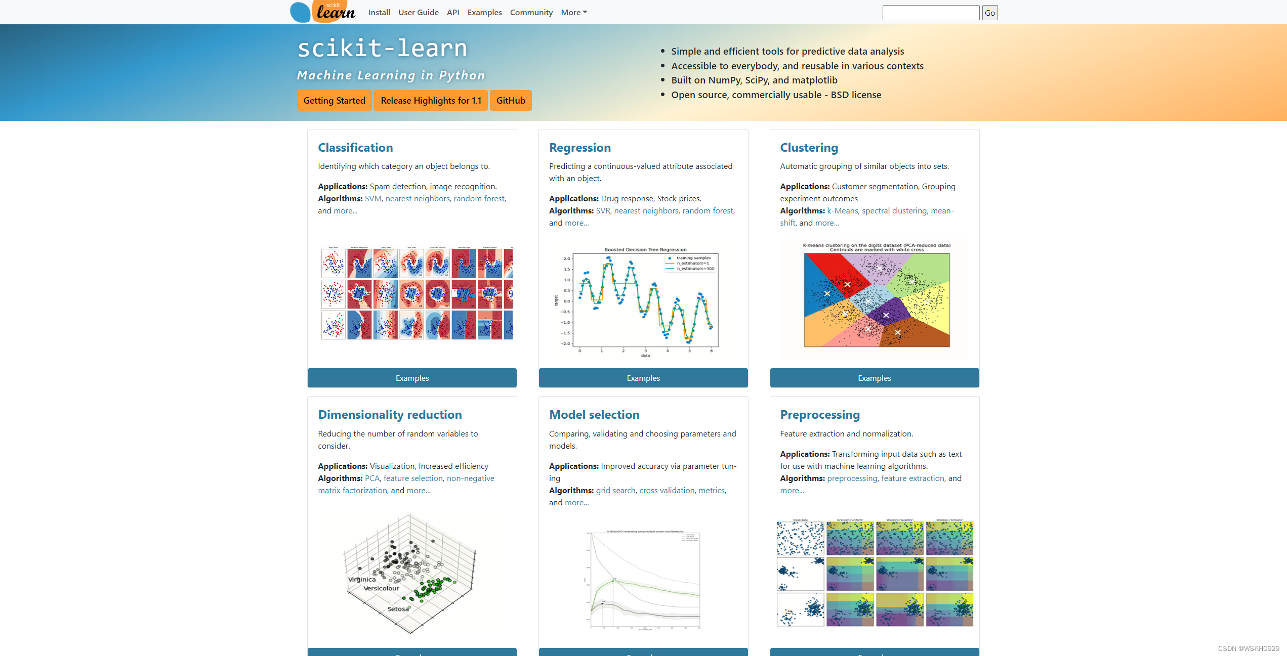
一、scikit-learn 工具包介绍

Scikit-learn（前身为scikits.learn，也称为sklearn）是一个用于Python编程语言的免费软件机器学习库。它具有各种分类、回归和聚类算法，包括支持向量机、随机森林、梯度提升、k-means和DBSCAN，并且设计用于与Python数字和科学库NumPy和SciPy互操作。Scikit learn是NumFOCUS财政资助的项目。

scikit-learn官网

scikit-learn 的安装也很简单。直接 pip install 即可

pip install scikit-learn

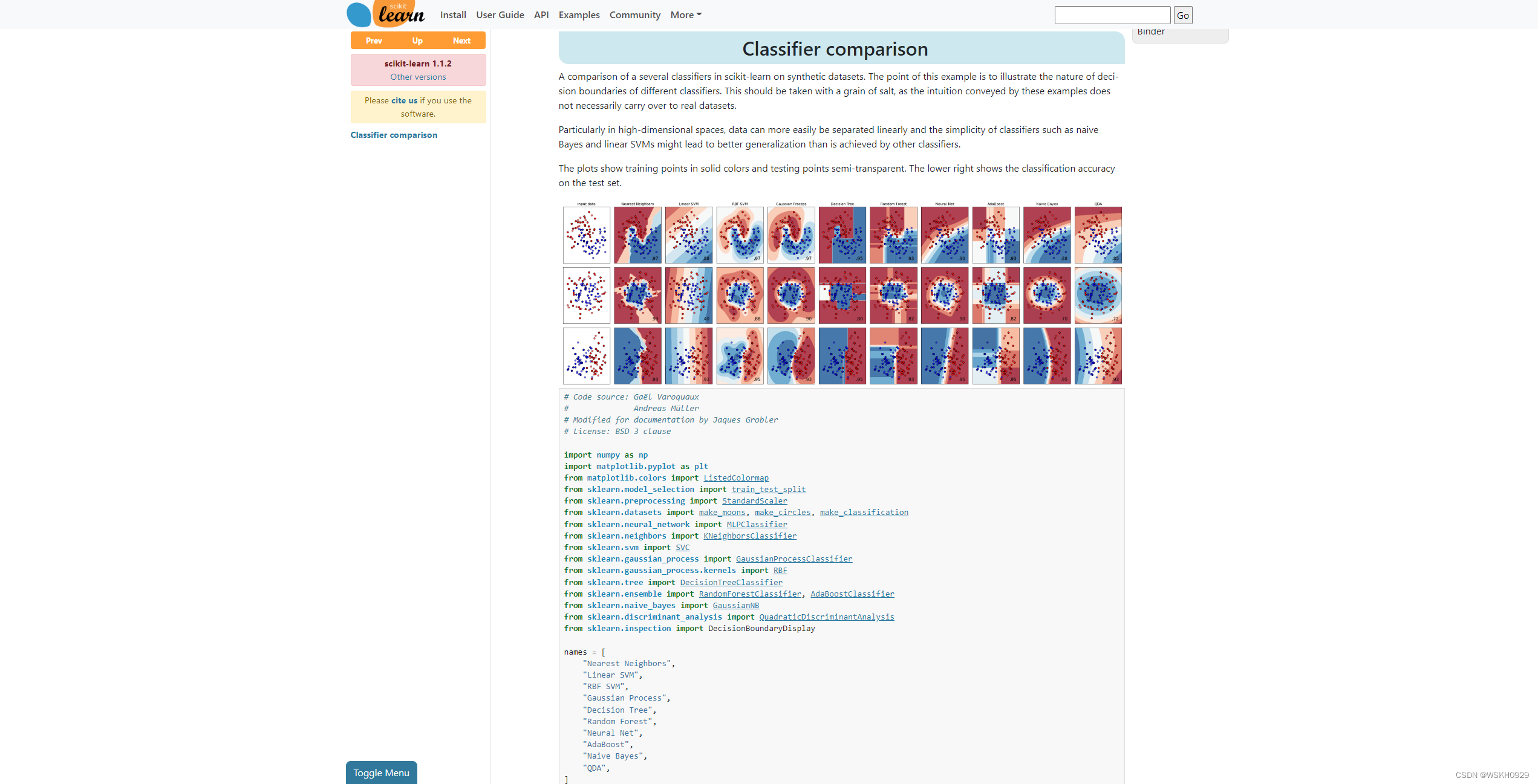
在官网顶部的Examples栏中，我们可以看到很多可视化的案例，当我们需要对结果进行可视化的时候，可以参考一下他们的可视化（真的很好看！）

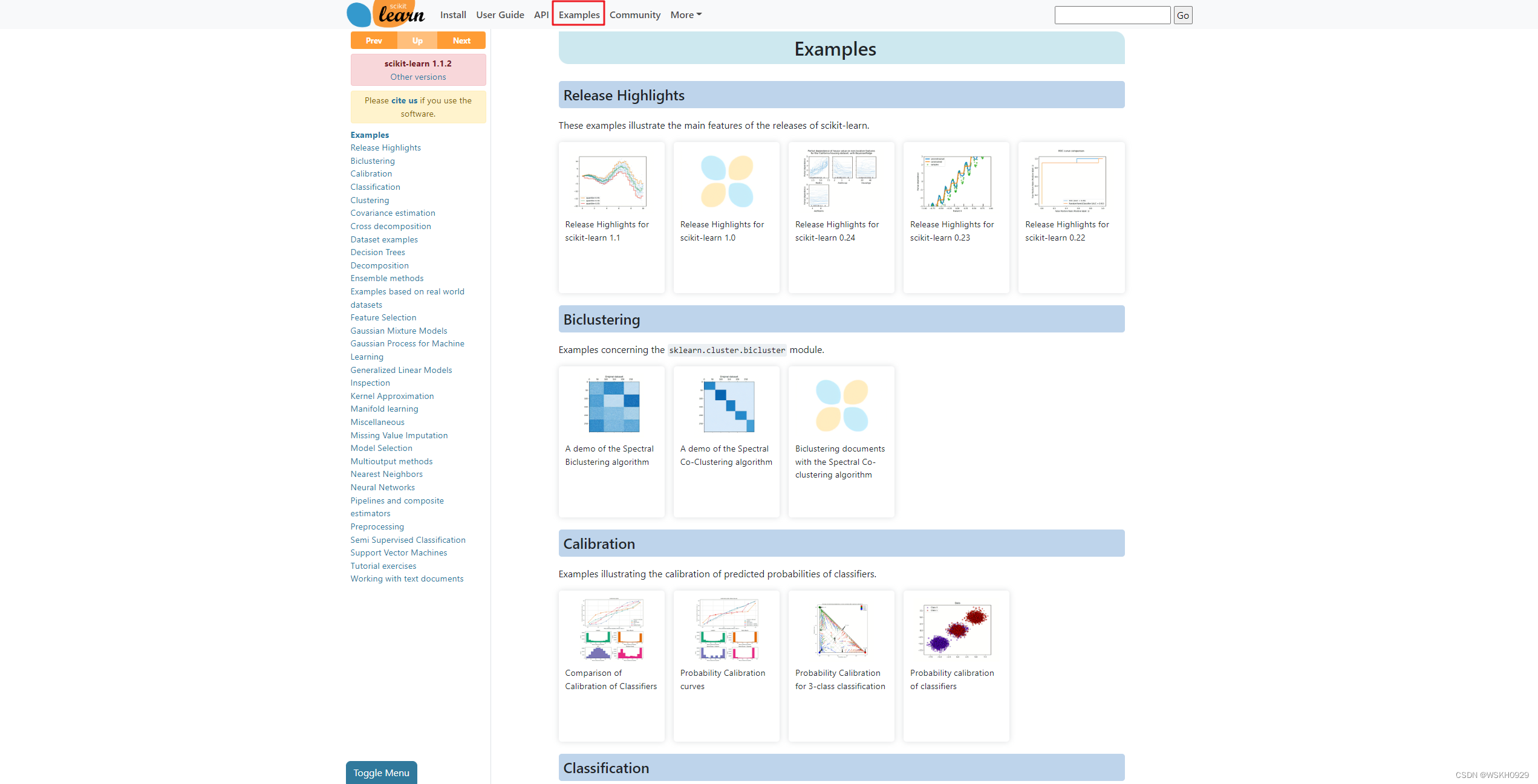
甚至还有代码可以直接复制

二、数据集划分

2.1 导入相关库

# 导入相关库
import numpy as np
import os
%matplotlib inline
import matplotlib
import matplotlib.pyplot as plt
from sklearn.datasets import fetch_openml

plt.rcParams['axes.labelsize'] = 14
plt.rcParams['xtick.labelsize'] = 12
plt.rcParams['ytick.labelsize'] = 12
import warnings

warnings.filterwarnings('ignore')
np.random.seed(42)

2.2 数据集读取

mnist = fetch_openml('mnist_784')

X,y = mnist["data"],mnist["target"]
print(X.shape)
print(y.shape)

输出：

(70000, 784)
(70000,)

2.3 划分训练集和测试集

X_train, X_test, y_train, y_test = train_test_split(X, y, test_size=0.3, random_state=520)
print(X_train.shape,X_test.shape)
print(y_train.shape,y_test.shape)

输出：

(49000, 784) (21000, 784)
(49000,) (21000,)

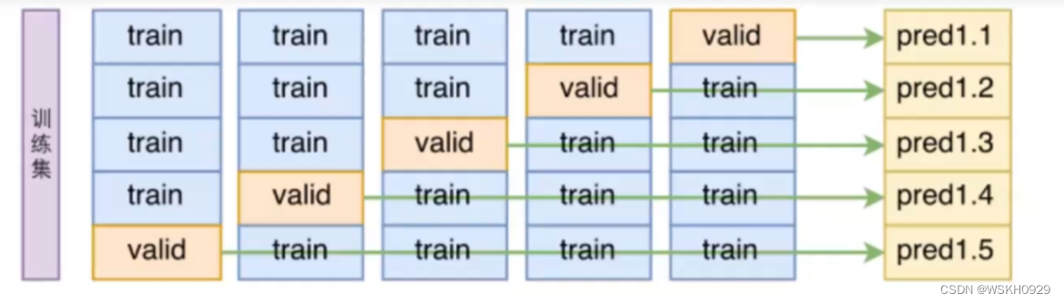
三、交叉验证

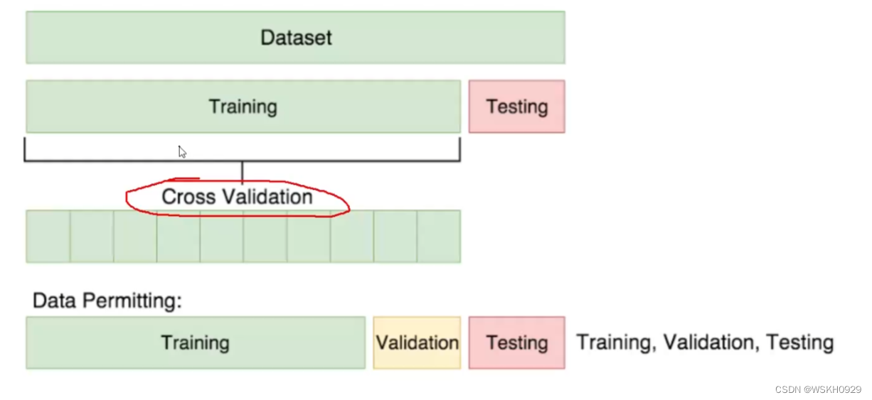
3.1 交叉验证的作用

• 正常机器学习流程中，我们会把原始数据划分为训练集和测试集，测试集作为最后对模型检验的标准。
• 可见测试集就和高考一样，非常重要，只有一次，在此之前，机器学习模型只能在训练集中进行训练和学习
• 但是机器也需要考试来检验他们自己的学习情况呀，但他们又只有训练集可以利用，怎么办呢？

交叉验证就可以解决机器学习模型需要”考试“的问题。即将训练集中的一部分数据作为验证集对机器学习进行验证，起到考试的作用。

3.2 交叉验证实验分析

先将标签转化为二类别，使得问题变为二分类问题

y_train_5 = (y_train == '5')
y_test_5 = (y_test == '5')

实例化SGD模型对象

from sklearn.linear_model import SGDClassifier

sgd_clf = SGDClassifier(max_iter=50,random_state=520)
sgd_clf.fit(X_train,y_train_5)

调用sklearn的库进行交叉验证

from sklearn.model_selection import cross_val_score
# 3折交叉验证
cross_val_score(sgd_clf, X_train, y_train_5, cv=3, scoring='accuracy')

输出（每一次交叉验证的准确率）：

array([0.969389  , 0.96369314, 0.95248883])

自己实现交叉验证

from sklearn.model_selection import StratifiedKFold
from sklearn.base import clone

# K折抽取数据的对象
skflods = StratifiedKFold(n_splits=3, random_state=520 , shuffle= True)

for train_index, test_index in skflods.split(X_train, y_train_5):
    # 将模型克隆一份
    clone_clf = clone(sgd_clf)
    # 将训练集划分为更小的训练集和验证集
    X_train_folds = X_train.iloc[train_index]
    y_train_folds = y_train_5.iloc[train_index]
    X_test_folds = X_train.iloc[test_index]
    y_test_folds = y_train_5.iloc[test_index]
    # 训练克隆的模型
    clone_clf.fit(X_train_folds, y_train_folds)
    # 进行预测
    y_pred = clone_clf.predict(X_test_folds)
    # 计算当前交叉验证的预测正确的样本数
    n_correct = sum(y_pred==y_test_folds)
    # 输出当前交叉验证的准确率
    print(n_correct / len(y_pred))

输出：

0.9691441165666708
0.9682850670421845
0.9622849445907059

四、混淆矩阵

from sklearn.model_selection import cross_val_predict

y_train_pred = cross_val_predict(sgd_clf,X_train,y_train_5,cv = 3)

print(y_train_pred.shape)
print(X_train.shape)

from sklearn.metrics import confusion_matrix

confusion_matrix(y_train_5,y_train_pred)

输出：

(49000,)
(49000, 784)
array([[43698,   814],
       [ 1055,  3433]], dtype=int64)

negative class [[ true negatives, false positives ],
positive class [ false negatives, true positives ]]

• true negatives: 43698 个数据被正确的分为非 5 类别
• false positives: 814 个数据被错误的分为 5 类别
• false negatives: 1055 个数据错误的分为非 5 类别
• true positives: 3433 个数据被正确的分为 5 类别

一个完美的分类器应该只有 true positives 和 true negatives, 即主对角线元素不为 0 ，其余元素为 0

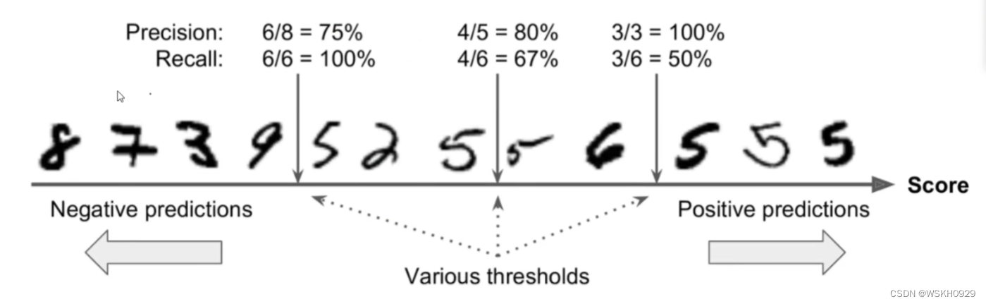
五、一些评估指标

from sklearn.metrics import precision_score,recall_score
# 准确率
print("precision_score:",precision_score(y_train_5,y_train_pred))
# 召回率
print("recall_score:",recall_score(y_train_5,y_train_pred))
# F1分数
print("f1_score:",f1_score(y_train_5,y_train_pred))

输出：

precision_score: 0.8083352955027078
recall_score: 0.7649286987522281
f1_score: 0.786033199771036

六、阈值对结果的影响

我们可以给模型的分类结果进行评分，然后指定阈值，根据阈值判断其所属类别

y_scores = sgd_clf.decision_function([X.iloc[35000]])
print(y_scores)
# 指定阈值t
t = -20000
# 根据阈值得到分类结果
y_pred = (y_scores >= t)
print(y_pred)

输出：

[-24367.70334503]
[False]

七、ROC曲线

receiver operating characteristic(ROC)曲线是二元分类中的常用评估方法

• 它与精确度/召回曲线非常相似，但ROC曲线不是绘制精确度与召回率，而是绘制true positive rate(TPR)与false positive rate(FPR)
• 要绘制ROC曲线，首先需要使用roc_curve()函数计算各种阈值的TPR和FPR:
• TPR TP /(TP FN)(Recall)
• FPR=FP/(FP TN)

from sklearn.metrics import roc_curve

y_scores = sgd_clf.decision_function(X_train)
fpr, tpr, thresholds = roc_curve(y_train_5, y_scores)


def plot_roc_curve(fpr, tpr, label=None):
    plt.plot(fpr, tpr, linewidth=2, label=label)
    plt.plot([0, 1], [0, 1], 'k--')
    plt.axis([0, 1, 0, 1])
    plt.xlabel('False Positive Rate', fontsize=16)
    plt.ylabel('True Positive Rate', fontsize=16)


plt.figure(figsize=(8, 6))
plot_roc_curve(fpr, tpr)
plt.show()

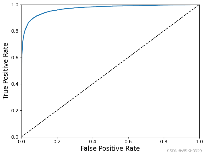
虚线表示纯随机分类器的ROC曲线；一个好的分类器尽可能远离该线（朝左上角）。比较分类器的一种方法是测量曲线下面积(AUC)。完美分类器的ROC AUC等于1，而纯随机分类器的ROC AUC等于0.5。Scikit-Learn提供了计算ROC AUC的函数：

from sklearn.metrics import roc_auc_score
roc_auc_score(y_train_5,y_scores)

输出：

0.9690493694904599