第9章逻辑回归

CaiGbro

已于 2022-11-05 19:52:54 修改

阅读量638

点赞数 2

分类专栏：机器学习笔记文章标签：逻辑回归 python 人工智能

于 2022-10-29 16:52:11 首次发布

本文链接：https://blog.csdn.net/weixin_52449030/article/details/127589069

版权

机器学习笔记专栏收录该内容

17 篇文章 1 订阅

订阅专栏

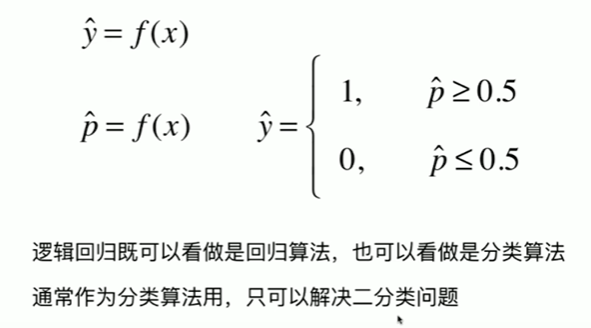
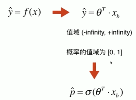
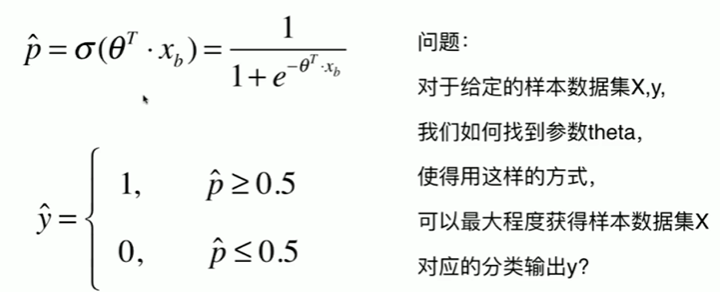
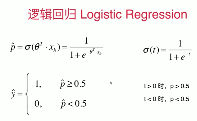
9-1 什么是逻辑回归

Notbook 示例

Notbook 源码

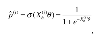
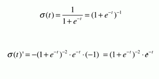
Sigmoid 函数
[1]
import numpy as np
import matplotlib.pyplot as plt
[2]
def sigmoid(t):
    return 1 / (1 + np.exp(-t))
[3]
X = np.linspace(-10,10,500)
y = sigmoid(X)

plt.plot(X,y)
[<matplotlib.lines.Line2D at 0x18b21371c40>]

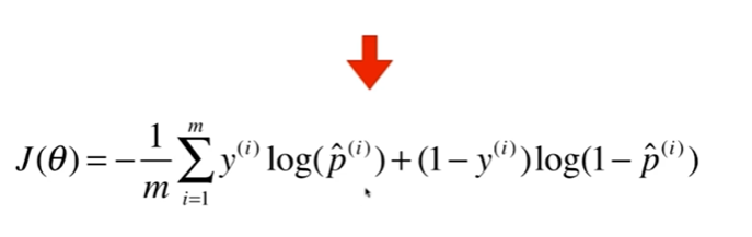
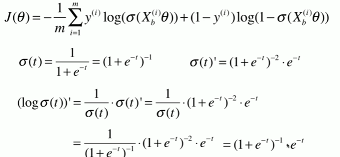
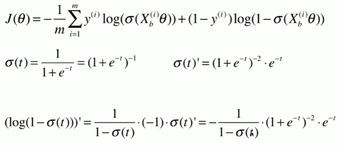
9-2 逻辑回归的损失函数

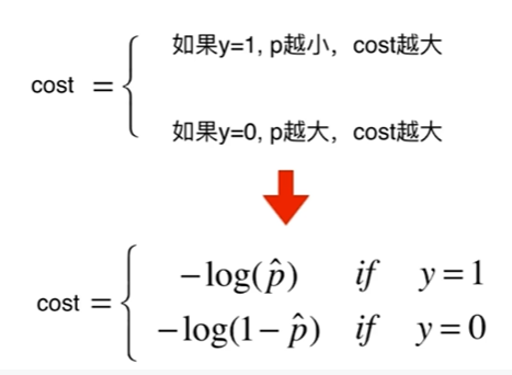
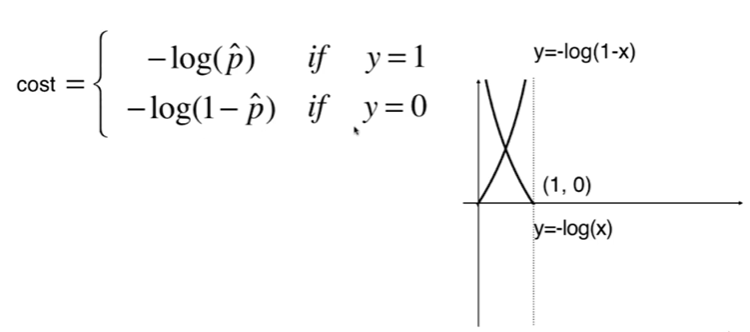
这里的cost表达式的意思是：

如果预测的值1或者0的可能性(准确度)越大，

那么cost就越小，可能性越小cost就越大，

所以要使拟合效果越好，就要让cost越小

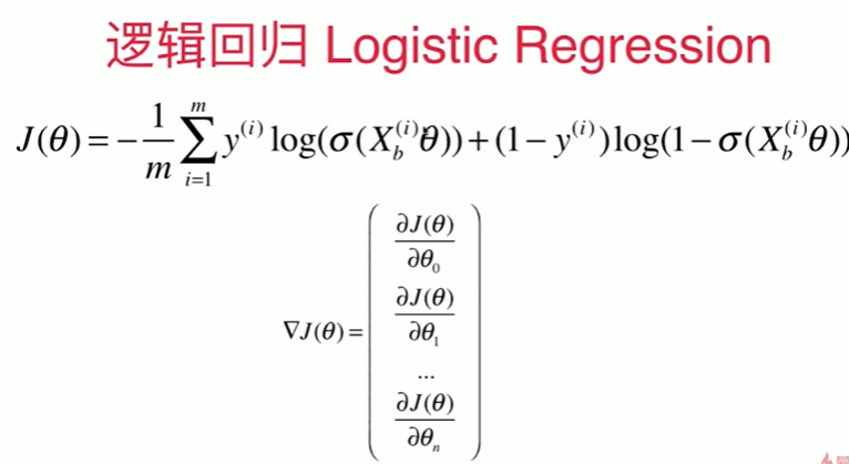
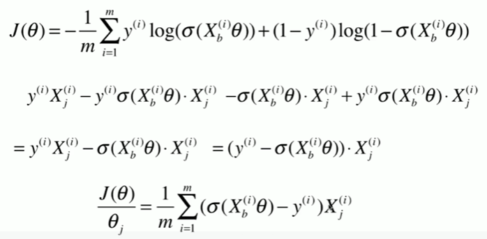
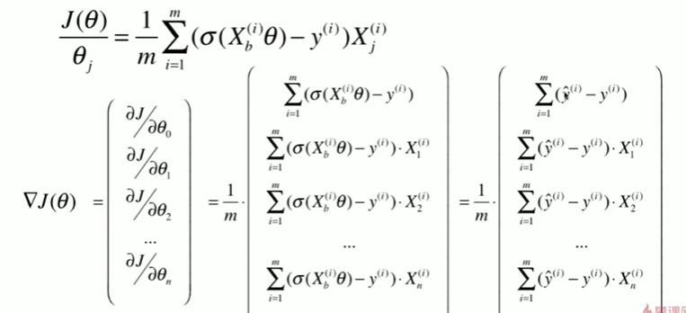
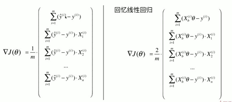
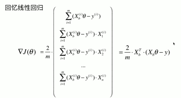
9-3 逻辑回归损失函数的梯度

9-4 and 9-5 实现逻辑回归算法与决策边界

Notbook 示例

Notbook 源码

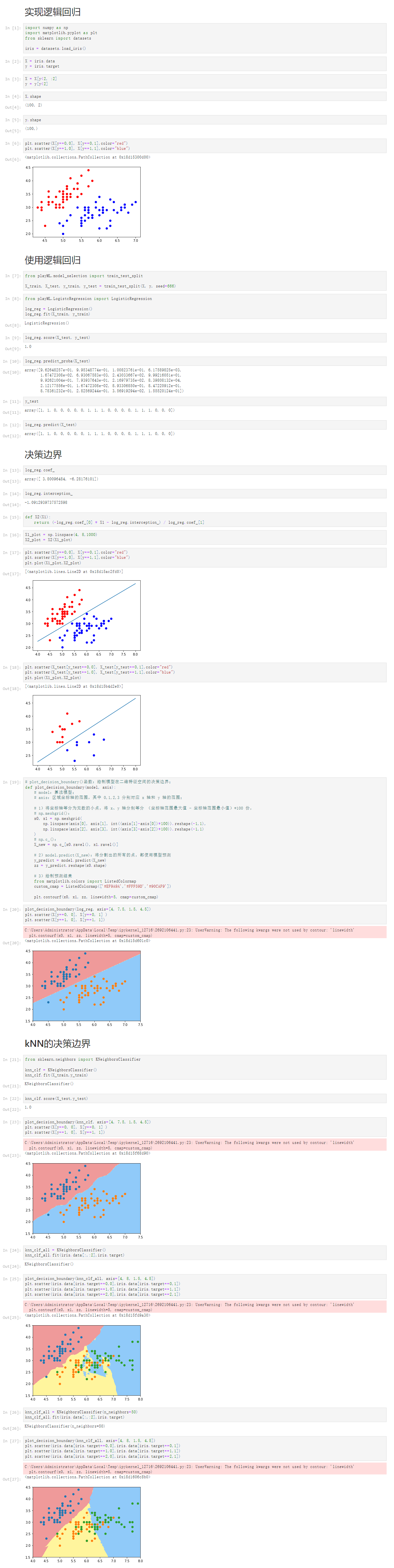
实现逻辑回归
[1]
import numpy as np 
import matplotlib.pyplot as plt
from sklearn import datasets

iris = datasets.load_iris()
[2]
X = iris.data
y = iris.target
[3]
X = X[y<2, :2]
y = y[y<2]
[4]
X.shape
(100, 2)
[5]
y.shape
(100,)
[6]
plt.scatter(X[y==0,0], X[y==0,1],color="red")
plt.scatter(X[y==1,0], X[y==1,1],color="blue")
<matplotlib.collections.PathCollection at 0x18d15300d00>

使用逻辑回归
[7]
from playML.model_selection import train_test_split

X_train, X_test, y_train, y_test = train_test_split(X, y, seed=666)
[8]
from playML.LogistcRegression import LogisticRegression

log_reg = LogisticRegression()
log_reg.fit(X_train, y_train)
LogisticRegression()
[9]
log_reg.score(X_test, y_test)
1.0
[10]
log_reg.predict_proba(X_test)
array([9.62648257e-01, 9.95348774e-01, 1.00823761e-01, 6.17589825e-03,
       1.67472308e-02, 6.93067583e-03, 2.43033667e-02, 9.99216051e-01,
       9.92621004e-01, 7.93937643e-01, 2.16979735e-02, 8.39808132e-04,
       2.12177556e-01, 1.67472308e-02, 8.93306850e-01, 8.47220912e-01,
       8.78361232e-01, 2.82569244e-01, 3.56919294e-02, 1.55520124e-01])
[11]
y_test
array([1, 1, 0, 0, 0, 0, 0, 1, 1, 1, 0, 0, 0, 0, 1, 1, 1, 0, 0, 0])
[12]
log_reg.predict(X_test)
array([1, 1, 0, 0, 0, 0, 0, 1, 1, 1, 0, 0, 0, 0, 1, 1, 1, 0, 0, 0])
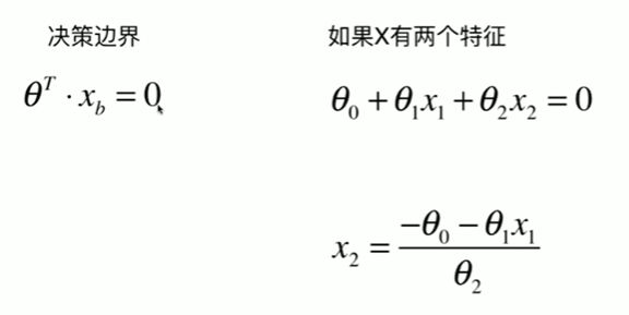
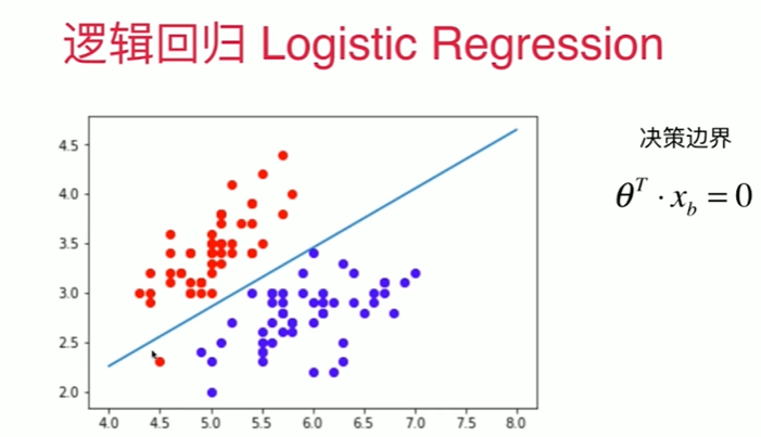
决策边界
[13]
log_reg.coef_
array([ 3.80096484, -6.28176101])
[14]
log_reg.interception_
-1.0912939737572598
[15]
def X2(X1):
    return (-log_reg.coef_[0] * X1 - log_reg.interception_) / log_reg.coef_[1]
[16]
X1_plot = np.linspace(4, 8,1000)
X2_plot = X2(X1_plot)
[17]
plt.scatter(X[y==0,0], X[y==0,1],color="red")
plt.scatter(X[y==1,0], X[y==1,1],color="blue")
plt.plot(X1_plot,X2_plot)
[<matplotlib.lines.Line2D at 0x18d15ac2fd0>]

[18]
plt.scatter(X_test[y_test==0,0], X_test[y_test==0,1],color="red")
plt.scatter(X_test[y_test==1,0], X_test[y_test==1,1],color="blue")
plt.plot(X1_plot,X2_plot)
[<matplotlib.lines.Line2D at 0x18d15b4d2e0>]

[19]
# plot_decision_boundary()函数：绘制模型在二维特征空间的决策边界；
def plot_decision_boundary(model, axis):
    # model：算法模型；
    # axis：区域坐标轴的范围，其中 0,1,2,3 分别对应 x 轴和 y 轴的范围；
    
    # 1）将坐标轴等分为无数的小点，将 x、y 轴分别等分 （坐标轴范围最大值 - 坐标轴范围最小值）*100 份，
    # np.meshgrid()：
    x0, x1 = np.meshgrid(
        np.linspace(axis[0], axis[1], int((axis[1]-axis[0])*100)).reshape(-1,1),
        np.linspace(axis[2], axis[3], int((axis[3]-axis[2])*100)).reshape(-1,1)
    )
    # np.c_()：
    X_new = np.c_[x0.ravel(), x1.ravel()]
    
    # 2）model.predict(X_new)：将分割出的所有的点，都使用模型预测
    y_predict = model.predict(X_new)
    zz = y_predict.reshape(x0.shape)
    
    # 3）绘制预测结果
    from matplotlib.colors import ListedColormap
    custom_cmap = ListedColormap(['#EF9A9A','#FFF59D','#90CAF9'])
    
    plt.contourf(x0, x1, zz, linewidth=5, cmap=custom_cmap)
[20]
plot_decision_boundary(log_reg, axis=[4, 7.5, 1.5, 4.5])
plt.scatter(X[y==0, 0], X[y==0, 1] )
plt.scatter(X[y==1, 0], X[y==1, 1])
C:\Users\Administrator\AppData\Local\Temp\ipykernel_12716\2692106441.py:23: UserWarning: The following kwargs were not used by contour: 'linewidth'
  plt.contourf(x0, x1, zz, linewidth=5, cmap=custom_cmap)

<matplotlib.collections.PathCollection at 0x18d15d601c0>

kNN的决策边界
[21]
from sklearn.neighbors import KNeighborsClassifier

knn_clf = KNeighborsClassifier()
knn_clf.fit(X_train,y_train)
KNeighborsClassifier()
[22]
knn_clf.score(X_test,y_test)
1.0
[23]
plot_decision_boundary(knn_clf, axis=[4, 7.5, 1.5, 4.5])
plt.scatter(X[y==0, 0], X[y==0, 1] )
plt.scatter(X[y==1, 0], X[y==1, 1])
C:\Users\Administrator\AppData\Local\Temp\ipykernel_12716\2692106441.py:23: UserWarning: The following kwargs were not used by contour: 'linewidth'
  plt.contourf(x0, x1, zz, linewidth=5, cmap=custom_cmap)

<matplotlib.collections.PathCollection at 0x18d15f68d90>

[24]
knn_clf_all = KNeighborsClassifier()
knn_clf_all.fit(iris.data[:,:2],iris.target)
KNeighborsClassifier()
[25]
plot_decision_boundary(knn_clf_all, axis=[4, 8, 1.5, 4.5])
plt.scatter(iris.data[iris.target==0,0],iris.data[iris.target==0,1])
plt.scatter(iris.data[iris.target==1,0],iris.data[iris.target==1,1])
plt.scatter(iris.data[iris.target==2,0],iris.data[iris.target==2,1])
C:\Users\Administrator\AppData\Local\Temp\ipykernel_12716\2692106441.py:23: UserWarning: The following kwargs were not used by contour: 'linewidth'
  plt.contourf(x0, x1, zz, linewidth=5, cmap=custom_cmap)

<matplotlib.collections.PathCollection at 0x18d15fd9a30>

[26]
knn_clf_all = KNeighborsClassifier(n_neighbors=50)
knn_clf_all.fit(iris.data[:,:2],iris.target)
KNeighborsClassifier(n_neighbors=50)
[27]
plot_decision_boundary(knn_clf_all, axis=[4, 8, 1.5, 4.5])
plt.scatter(iris.data[iris.target==0,0],iris.data[iris.target==0,1])
plt.scatter(iris.data[iris.target==1,0],iris.data[iris.target==1,1])
plt.scatter(iris.data[iris.target==2,0],iris.data[iris.target==2,1])
C:\Users\Administrator\AppData\Local\Temp\ipykernel_12716\2692106441.py:23: UserWarning: The following kwargs were not used by contour: 'linewidth'
  plt.contourf(x0, x1, zz, linewidth=5, cmap=custom_cmap)

<matplotlib.collections.PathCollection at 0x18d1606c8b0>

9-6 在逻辑回归中使用多项式特征

Notbook 示例

Notbook 源码

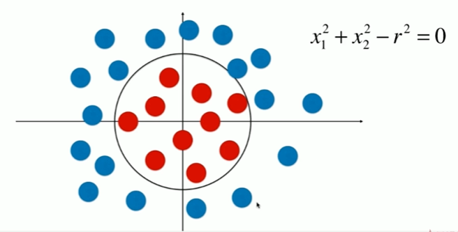
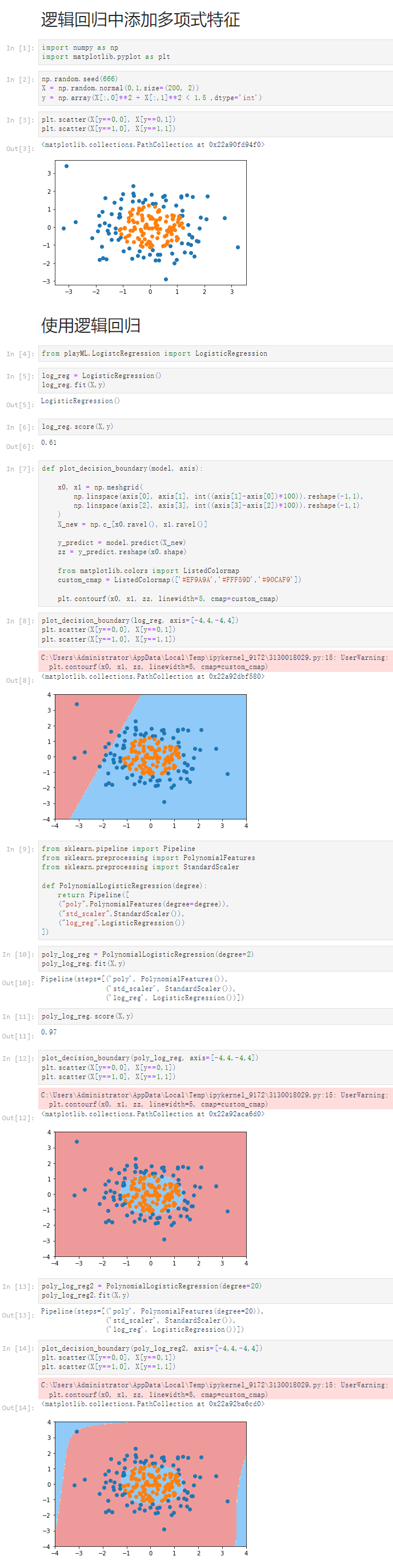
逻辑回归中添加多项式特征
[1]
import numpy as np
import matplotlib.pyplot as plt
[2]
np.random.seed(666)
X = np.random.normal(0,1,size=(200, 2))
y = np.array(X[:,0]**2 + X[:,1]**2 < 1.5 ,dtype='int')
[3]
plt.scatter(X[y==0,0], X[y==0,1])
plt.scatter(X[y==1,0], X[y==1,1])
<matplotlib.collections.PathCollection at 0x22a90fd94f0>

使用逻辑回归
[4]
from playML.LogistcRegression import LogisticRegression
[5]
log_reg = LogisticRegression()
log_reg.fit(X,y)
LogisticRegression()
[6]
log_reg.score(X,y)
0.61
[7]
def plot_decision_boundary(model, axis):

    x0, x1 = np.meshgrid(
        np.linspace(axis[0], axis[1], int((axis[1]-axis[0])*100)).reshape(-1,1),
        np.linspace(axis[2], axis[3], int((axis[3]-axis[2])*100)).reshape(-1,1)
    )
    X_new = np.c_[x0.ravel(), x1.ravel()]
    
    y_predict = model.predict(X_new)
    zz = y_predict.reshape(x0.shape)

    from matplotlib.colors import ListedColormap
    custom_cmap = ListedColormap(['#EF9A9A','#FFF59D','#90CAF9'])
    
    plt.contourf(x0, x1, zz, linewidth=5, cmap=custom_cmap)
[8]
plot_decision_boundary(log_reg, axis=[-4,4,-4,4])
plt.scatter(X[y==0,0], X[y==0,1])
plt.scatter(X[y==1,0], X[y==1,1])
C:\Users\Administrator\AppData\Local\Temp\ipykernel_9172\3130018029.py:15: UserWarning: The following kwargs were not used by contour: 'linewidth'
  plt.contourf(x0, x1, zz, linewidth=5, cmap=custom_cmap)

<matplotlib.collections.PathCollection at 0x22a92dbf580>

[9]
from sklearn.pipeline import Pipeline
from sklearn.preprocessing import PolynomialFeatures
from sklearn.preprocessing import StandardScaler

def PolynomialLogisticRegression(degree):
    return Pipeline([
    ("poly",PolynomialFeatures(degree=degree)),
    ("std_scaler",StandardScaler()),
    ("log_reg",LogisticRegression())
])
[10]
poly_log_reg = PolynomialLogisticRegression(degree=2)
poly_log_reg.fit(X,y)
Pipeline(steps=[('poly', PolynomialFeatures()),
                ('std_scaler', StandardScaler()),
                ('log_reg', LogisticRegression())])
[11]
poly_log_reg.score(X,y)
0.97
[12]
plot_decision_boundary(poly_log_reg, axis=[-4,4,-4,4])
plt.scatter(X[y==0,0], X[y==0,1])
plt.scatter(X[y==1,0], X[y==1,1])
C:\Users\Administrator\AppData\Local\Temp\ipykernel_9172\3130018029.py:15: UserWarning: The following kwargs were not used by contour: 'linewidth'
  plt.contourf(x0, x1, zz, linewidth=5, cmap=custom_cmap)

<matplotlib.collections.PathCollection at 0x22a92aca6d0>

[13]
poly_log_reg2 = PolynomialLogisticRegression(degree=20)
poly_log_reg2.fit(X,y)
Pipeline(steps=[('poly', PolynomialFeatures(degree=20)),
                ('std_scaler', StandardScaler()),
                ('log_reg', LogisticRegression())])
[14]
plot_decision_boundary(poly_log_reg2, axis=[-4,4,-4,4])
plt.scatter(X[y==0,0], X[y==0,1])
plt.scatter(X[y==1,0], X[y==1,1])
C:\Users\Administrator\AppData\Local\Temp\ipykernel_9172\3130018029.py:15: UserWarning: The following kwargs were not used by contour: 'linewidth'
  plt.contourf(x0, x1, zz, linewidth=5, cmap=custom_cmap)

<matplotlib.collections.PathCollection at 0x22a92ba6cd0>

9-7 scikit-learn中的逻辑回归

Notbook 示例

Notbook 源码

[1]
import numpy as np
import matplotlib.pyplot as plt
[2]
np.random.seed(666)
X = np.random.normal(0,1,size=(200, 2))
y = np.array(X[:,0]**2 + X[:,1] < 1.5 ,dtype='int')
for _ in range(20):
    y[np.random.randint(200)] = 1
[3]
plt.scatter(X[y==0,0], X[y==0,1])
plt.scatter(X[y==1,0], X[y==1,1])
<matplotlib.collections.PathCollection at 0x2397e35b220>

[4]
from sklearn.model_selection import train_test_split
X_train, X_test, y_train, y_test = train_test_split(X, y,random_state=666)
使用scikit-learn 中的逻辑回归
[5]
from sklearn.linear_model import LogisticRegression

log_reg = LogisticRegression()
log_reg.fit(X_train, y_train)
LogisticRegression()
[6]
log_reg.score(X_train,y_train)
0.7933333333333333
[7]
log_reg.score(X_test,y_test)
0.86
[8]
def plot_decision_boundary(model, axis):

    x0, x1 = np.meshgrid(
        np.linspace(axis[0], axis[1], int((axis[1]-axis[0])*100)).reshape(-1,1),
        np.linspace(axis[2], axis[3], int((axis[3]-axis[2])*100)).reshape(-1,1)
    )
    X_new = np.c_[x0.ravel(), x1.ravel()]
    
    y_predict = model.predict(X_new)
    zz = y_predict.reshape(x0.shape)

    from matplotlib.colors import ListedColormap
    custom_cmap = ListedColormap(['#EF9A9A','#FFF59D','#90CAF9'])
    
    plt.contourf(x0, x1, zz, linewidth=5, cmap=custom_cmap)
[9]
plot_decision_boundary(log_reg, axis=[-4,4,-4,4])
plt.scatter(X[y==0,0], X[y==0,1])
plt.scatter(X[y==1,0], X[y==1,1])
C:\Users\Administrator\AppData\Local\Temp\ipykernel_13668\3130018029.py:15: UserWarning: The following kwargs were not used by contour: 'linewidth'
  plt.contourf(x0, x1, zz, linewidth=5, cmap=custom_cmap)

<matplotlib.collections.PathCollection at 0x23903dc3460>

[10]
from sklearn.pipeline import Pipeline
from sklearn.preprocessing import PolynomialFeatures
from sklearn.preprocessing import StandardScaler

def PolynomialLogisticRegression(degree):
    return Pipeline([
    ("poly",PolynomialFeatures(degree=degree)),
    ("std_scaler",StandardScaler()),
    ("log_reg",LogisticRegression())
])
[11]
poly_log_reg = PolynomialLogisticRegression(degree=2)
poly_log_reg.fit(X_train,y_train)
Pipeline(steps=[('poly', PolynomialFeatures()),
                ('std_scaler', StandardScaler()),
                ('log_reg', LogisticRegression())])
[12]
poly_log_reg.score(X_train,y_train)
0.9066666666666666
[13]
poly_log_reg.score(X_test,y_test)
0.94
[14]
plot_decision_boundary(poly_log_reg, axis=[-4,4,-4,4])
plt.scatter(X[y==0,0], X[y==0,1])
plt.scatter(X[y==1,0], X[y==1,1])
C:\Users\Administrator\AppData\Local\Temp\ipykernel_13668\3130018029.py:15: UserWarning: The following kwargs were not used by contour: 'linewidth'
  plt.contourf(x0, x1, zz, linewidth=5, cmap=custom_cmap)

<matplotlib.collections.PathCollection at 0x23902a64790>

[15]
poly_log_reg2 = PolynomialLogisticRegression(degree=20)
poly_log_reg2.fit(X_train,y_train)
Pipeline(steps=[('poly', PolynomialFeatures(degree=20)),
                ('std_scaler', StandardScaler()),
                ('log_reg', LogisticRegression())])
[16]
poly_log_reg2.score(X_train,y_train)
0.94
[17]
poly_log_reg2.score(X_test,y_test)
0.92
[18]
plot_decision_boundary(poly_log_reg2, axis=[-4,4,-4,4])
plt.scatter(X[y==0,0], X[y==0,1])
plt.scatter(X[y==1,0], X[y==1,1])
C:\Users\Administrator\AppData\Local\Temp\ipykernel_13668\3130018029.py:15: UserWarning: The following kwargs were not used by contour: 'linewidth'
  plt.contourf(x0, x1, zz, linewidth=5, cmap=custom_cmap)

<matplotlib.collections.PathCollection at 0x239034965b0>

[19]
def PolynomialLogisticRegression(degree, C):
    return Pipeline([
    ("poly",PolynomialFeatures(degree=degree)),
    ("std_scaler",StandardScaler()),
    ("log_reg",LogisticRegression(C=C))
])
[20]
poly_log_reg3 = PolynomialLogisticRegression(degree=20, C=0.1)
poly_log_reg3.fit(X_train,y_train)
Pipeline(steps=[('poly', PolynomialFeatures(degree=20)),
                ('std_scaler', StandardScaler()),
                ('log_reg', LogisticRegression(C=0.1))])
[21]
poly_log_reg3.score(X_train,y_train)
0.84
[22]
poly_log_reg3.score(X_test,y_test)
0.92
[23]
plot_decision_boundary(poly_log_reg3, axis=[-4,4,-4,4])
plt.scatter(X[y==0,0], X[y==0,1])
plt.scatter(X[y==1,0], X[y==1,1])
C:\Users\Administrator\AppData\Local\Temp\ipykernel_13668\3130018029.py:15: UserWarning: The following kwargs were not used by contour: 'linewidth'
  plt.contourf(x0, x1, zz, linewidth=5, cmap=custom_cmap)

<matplotlib.collections.PathCollection at 0x23902feb970>

[24]
def PolynomialLogisticRegression(degree, C, penalty='l2'):
    return Pipeline([
    ("poly",PolynomialFeatures(degree=degree)),
    ("std_scaler",StandardScaler()),
    ("log_reg",LogisticRegression(C=C))
])
[25]
poly_log_reg4 = PolynomialLogisticRegression(degree=20,C=0.1,penalty='l1')
poly_log_reg4.fit(X_train,y_train)
Pipeline(steps=[('poly', PolynomialFeatures(degree=20)),
                ('std_scaler', StandardScaler()),
                ('log_reg', LogisticRegression(C=0.1))])
[26]
poly_log_reg4.score(X_train,y_train)
0.84
[27]
poly_log_reg4.score(X_test,y_test)
0.92
[28]
plot_decision_boundary(poly_log_reg4, axis=[-4,4,-4,4])
plt.scatter(X[y==0,0], X[y==0,1])
plt.scatter(X[y==1,0], X[y==1,1])
C:\Users\Administrator\AppData\Local\Temp\ipykernel_13668\3130018029.py:15: UserWarning: The following kwargs were not used by contour: 'linewidth'
  plt.contourf(x0, x1, zz, linewidth=5, cmap=custom_cmap)

<matplotlib.collections.PathCollection at 0x23902b3c760>

9-8 OvR与OvO

Notbook 示例

Notbook 源码

OvR 和 OvO
[1]
import numpy as np
import matplotlib.pyplot as plt
from sklearn import datasets

iris = datasets.load_iris()
X = iris.data[:, :2]
y = iris.target
[2]
from sklearn.model_selection import train_test_split

X_train, X_test, y_train, y_test = train_test_split(X, y,random_state=7)
[3]
from sklearn.linear_model import LogisticRegression

log_reg = LogisticRegression(multi_class="ovr")
log_reg.fit(X_train,y_train)
LogisticRegression(multi_class='ovr')
[4]
log_reg.score(X_test,y_test)
0.6052631578947368
[5]
def plot_decision_boundary(model, axis):

    x0, x1 = np.meshgrid(
        np.linspace(axis[0], axis[1], int((axis[1]-axis[0])*100)).reshape(-1,1),
        np.linspace(axis[2], axis[3], int((axis[3]-axis[2])*100)).reshape(-1,1)
    )
    X_new = np.c_[x0.ravel(), x1.ravel()]
    
    y_predict = model.predict(X_new)
    zz = y_predict.reshape(x0.shape)

    from matplotlib.colors import ListedColormap
    custom_cmap = ListedColormap(['#EF9A9A','#FFF59D','#90CAF9'])
    
    plt.contourf(x0, x1, zz, linewidth=5, cmap=custom_cmap)
[6]
plot_decision_boundary(log_reg, axis=[4,8.5,1.5,4.5])
plt.scatter(X[y==0,0], X[y==0,1])
plt.scatter(X[y==1,0], X[y==1,1])
plt.scatter(X[y==2,0], X[y==2,1])
C:\Users\Administrator\AppData\Local\Temp\ipykernel_8836\3130018029.py:15: UserWarning: The following kwargs were not used by contour: 'linewidth'
  plt.contourf(x0, x1, zz, linewidth=5, cmap=custom_cmap)

<matplotlib.collections.PathCollection at 0x277418551f0>

[7]
log_reg2 = LogisticRegression(multi_class="multinomial", solver='newton-cg')
[8]
log_reg2.fit(X_train, y_train)
log_reg2.score(X_test,y_test)
0.6842105263157895
[9]
plot_decision_boundary(log_reg2, axis=[4,8.5,1.5,4.5])
plt.scatter(X[y==0,0], X[y==0,1])
plt.scatter(X[y==1,0], X[y==1,1])
plt.scatter(X[y==2,0], X[y==2,1])
C:\Users\Administrator\AppData\Local\Temp\ipykernel_8836\3130018029.py:15: UserWarning: The following kwargs were not used by contour: 'linewidth'
  plt.contourf(x0, x1, zz, linewidth=5, cmap=custom_cmap)

<matplotlib.collections.PathCollection at 0x27741808880>

使用所有数据
[10]
X = iris.data
y = iris.target

from sklearn.model_selection import train_test_split

X_train, X_test, y_train, y_test = train_test_split(X, y,random_state=654)
[11]
log_reg = LogisticRegression(multi_class="ovr")
log_reg.fit(X_train, y_train)
log_reg.score(X_test,y_test)
0.9473684210526315
[12]
log_reg2 = LogisticRegression()
log_reg2.fit(X_train, y_train)
log_reg2.score(X_test,y_test)
0.9736842105263158
OvO and OvR
[13]
from sklearn.multiclass import OneVsRestClassifier

ovr =OneVsRestClassifier(log_reg)
ovr.fit(X_train,y_train)
ovr.score(X_test,y_test)
0.9473684210526315
[14]
from sklearn.multiclass import OneVsOneClassifier

ovo = OneVsOneClassifier(log_reg)
ovo.fit(X_train,y_train)
ovo.score(X_test,y_test)
0.9736842105263158