初识线性回归(Excel-Python实现)

目录
一.excel数据分析功能实现
二. jupyter实现
1.最小二乘法
平均值
参数a b
这里对参数保留4位有效数字
导入所需的模块
2.skleran库完成
三.总结
目录

一.excel数据分析功能实现
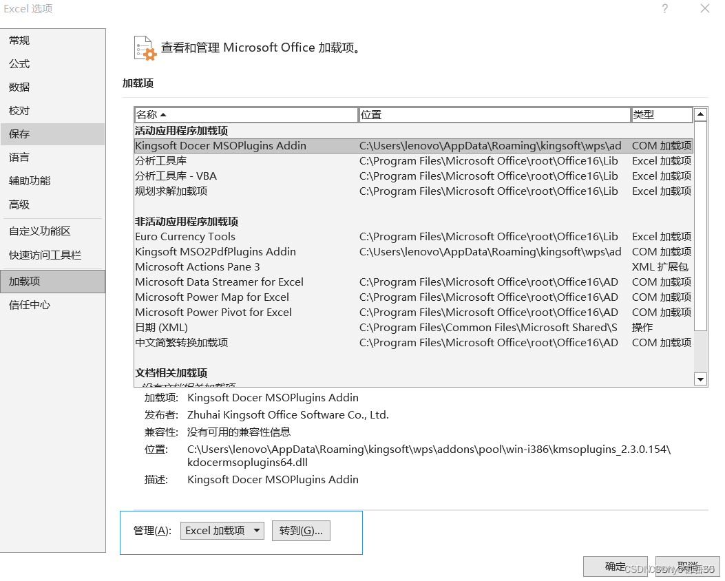
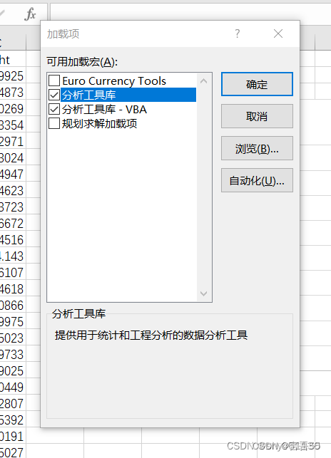
1.添加数据分析工具

在菜单栏选择“插入”，“我的加载项”，“管理其他加载项”，在最下方选择Excel加载项，点击“转到”：

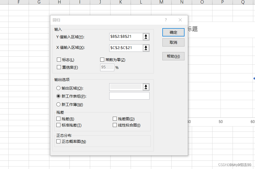
2.excel完成线性回归分析

数据-数据分析-回归

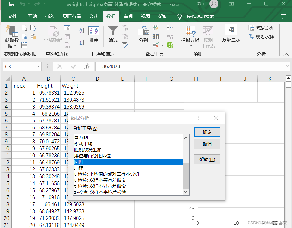
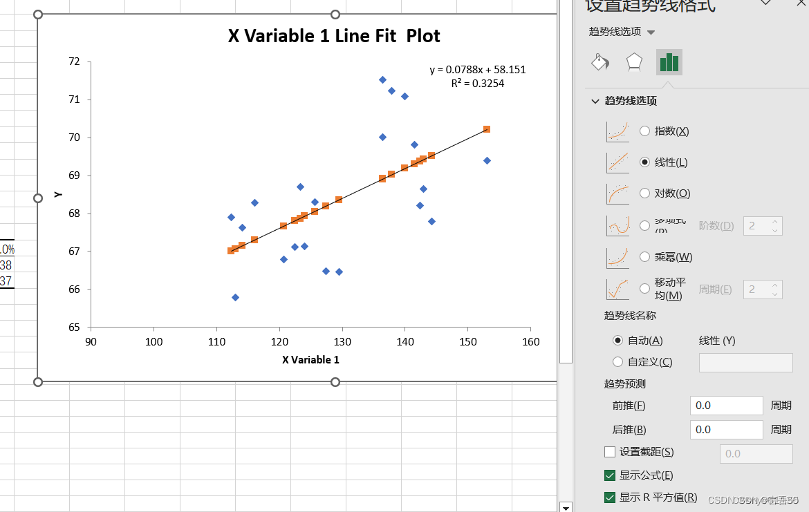
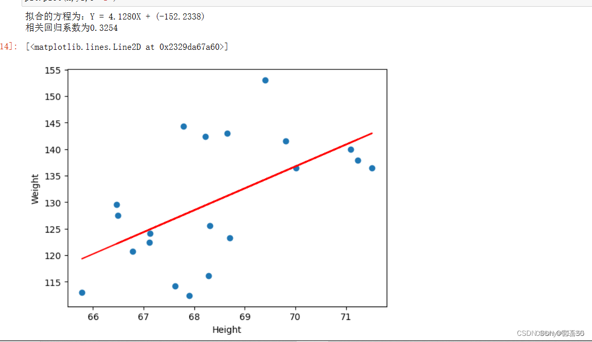
选择20组数据

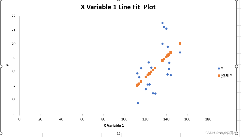
添加趋势线

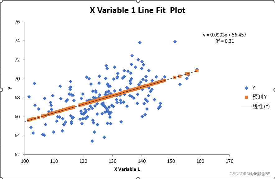
200组

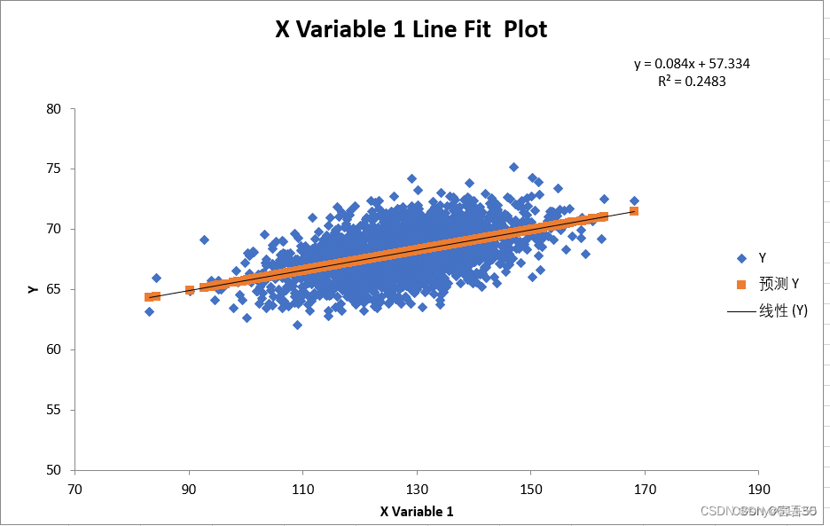
2000组

二. jupyter实现
1.最小二乘法
1.最小二乘法
将所需要的数据文件导入到jupyter中，就可以不用在程序里使用数据文件时加入路径。
打开jupyter，点击upload，选择你需要的文件，确定，点击上传

import pandas as pd
import numpy as np
import math
#准备数据
p=pd.read_excel('weights_heights(身高-体重数据集).xls','weights_heights')
#读取20行数据
p1=p.head(20)
x=p1["Height"]
y=p1["Weight"]
1
2
3
4
5
6
7
8
9

平均值

x_mean = np.mean(x)
y_mean = np.mean(y)
#x（或y）列的总数（即n）
xsize = x.size
zi=((x-x_mean)*(y-y_mean)).sum()
mu=((x-x_mean)*(x-x_mean)).sum()
n=((y-y_mean)*(y-y_mean)).sum()
1
2
3
4
5
6
7

参数a b

a = zi / mu
b = y_mean - a * x_mean
#相关系数R的平方
m=((zi/math.sqrt(mu*n))**2)
1
2
3
4

这里对参数保留4位有效数字

a = np.around(a,decimals=4)
b = np.around(b,decimals=4)
m = np.around(m,decimals=4)
print(f'回归线方程:y = {a}x +({b})') 
print(f'相关回归系数为{m}')
#借助第三方库skleran画出拟合曲线
y1 = a*x + b
plt.scatter(x,y)
plt.plot(x,y1,c='r')
1
2
3
4
5
6
7
8
9

20组数据

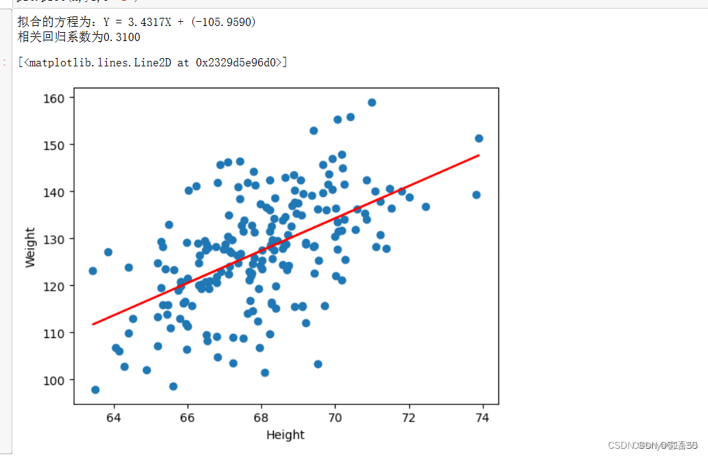
200组数据

2000组数据

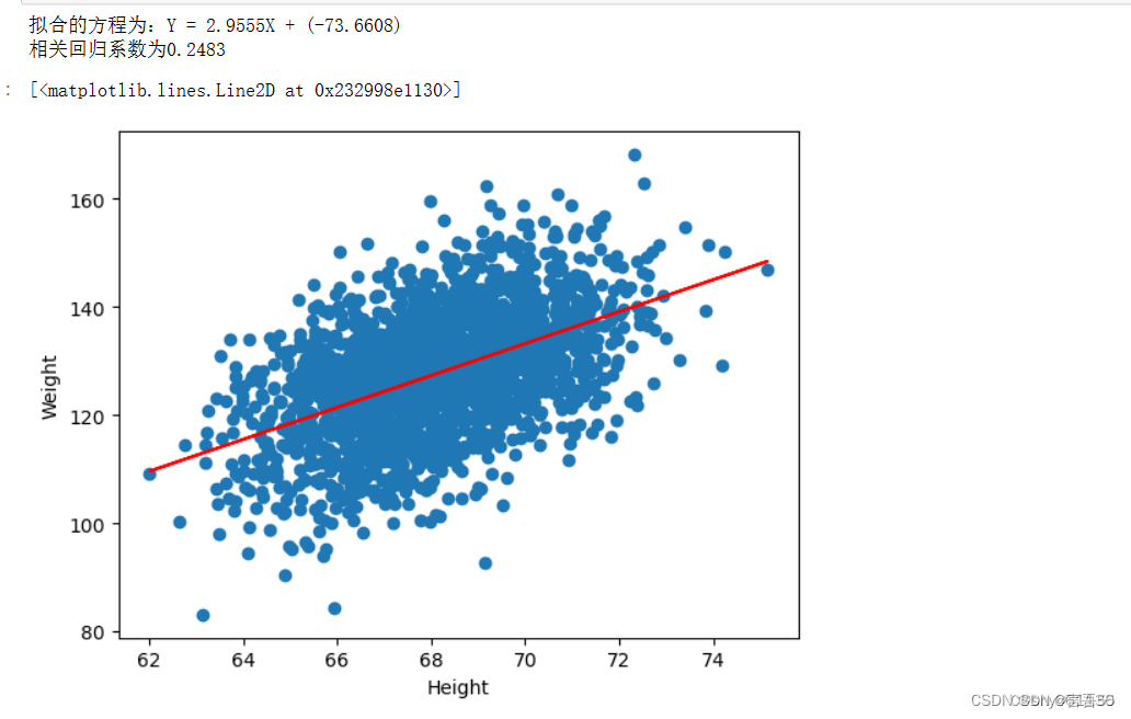
p1=p.head(20)改为p1=p.head(2000)

2.skleran库完成

导入所需的模块
import numpy as np
import pandas as pd
import matplotlib.pyplot as plt
from sklearn.linear_model import LinearRegression
 
p=pd.read_excel('weights_heights(身高-体重数据集).xls','weights_heights')
#读取数据行数
p1=p.head(20)
x=p1["Height"]
y=p1["Weight"]
1
2
3
4
5
6
7
8
9
10

```python
y = np.array(y).reshape(-1, 1)
x = np.array(x).reshape(-1, 1)
# 拟合

2.skleran库完成

prediction = reg.predict(y)                # 根据高度，按照拟合的曲线预测温度值
plt.xlabel('身高')
plt.ylabel('体重')
plt.scatter(x,y)
y1 = a*x + b
plt.plot(x,y1,c='r')

20组

200组

2000组

三.总结
excle和借助skleran库进行回归分析结果接近，都是借用调用现有的函数进行分析得到结果，操作简单。