有重叠部分的两张图融合还原（细胞图像融合以及拼接技术为例）

在图像处理领域，对于有重叠部分的两张图片的拼接还原，一直是一个热门且具有挑战性的研究课题。这种技术在很多领域都有广泛的应用，如全景摄影、虚拟现实、遥感图像处理等。随着科技的发展，对图像拼接还原的准确性和效率提出了更高的要求。

图像拼接还原的核心在于找到两张图片的重叠部分，并对其进行精确的配准和融合。常用的方法包括特征点匹配、变换模型估计、图像融合等。特征点匹配通过在两张图片中寻找相似的特征点，建立起它们之间的对应关系；变换模型估计则根据这些对应关系，计算出一个合适的变换模型，使得两张图片在重叠区域能够无缝拼接；最后，图像融合则负责将拼接后的图像进行平滑处理，消除拼接痕迹，使整体看起来更加自然

图像处理的具体步骤如下：

1.准备阶段：首先，需要收集有重叠部分的两张图片。这两张图片应具有一定的重叠区域，以便进行后续的还原操作。

2.图像预处理：对收集到的两张图片进行预处理，包括图像缩放、裁剪、旋转等操作，使得两张图片的重叠区域能够更好地对齐。

3.图像配准：通过图像配准算法，将两张图片的重叠区域进行对齐。这可以通过计算两张图片的重叠区域的特征点，然后利用这些特征点进行配准。配准完成后，两张图片的重叠区域应该能够完全对齐。

4.图像融合：在图像配准的基础上，进行图像融合操作。可以采用多种图像融合算法，如加权平均法、拉普拉斯金字塔融合法、小波变换融合法等。这些算法可以将两张图片的重叠区域进行融合，生成一张新的图片，该图片包含了两张图片的所有信息。

5.后处理：对融合后的图片进行后处理，包括去噪、锐化、色彩校正等操作，使得生成的图片质量更高。

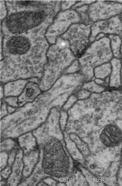
现以细胞图像融合以及拼接技术为例，展示具体的MATLAB仿真实现程序：

feature_based_panoramic_stitching_custom
function feature_based_panoramic_stitching_custom
    % Step 1 - Load specific Images
    files = {'E:\4.19\3.png', 'E:\4.19\4.png'};
    numImages = numel(files);
    tforms(numImages) = projective2d(eye(3));
    imageSize = zeros(numImages,2);

    % Read and display the first image
    I = imread(files{1});
    grayImage = im2gray(I);
    points = detectSURFFeatures(grayImage);
    [features, points] = extractFeatures(grayImage, points);

    % Initialize transformations and image sizes
    imageSize(1,:) = size(grayImage);

    for n = 2:numImages
        % Store points and features for I(n-1)
        pointsPrevious = points;
        featuresPrevious = features;

        % Read I(n)
        I = imread(files{n});
        grayImage = im2gray(I);
        imageSize(n,:) = size(grayImage);

        % Detect and extract SURF features for I(n)
        points = detectSURFFeatures(grayImage);
        [features, points] = extractFeatures(grayImage, points);

        % Find correspondences between I(n) and I(n-1)
        indexPairs = matchFeatures(features, featuresPrevious, 'Unique', true);
        matchedPoints = points(indexPairs(:,1), :);
        matchedPointsPrev = pointsPrevious(indexPairs(:,2), :);

        % Estimate the transformation between I(n) and I(n-1)
        tforms(n) = estimateGeometricTransform2D(matchedPoints, matchedPointsPrev,...
            'projective', 'Confidence', 99.9, 'MaxNumTrials', 2000);

        % Accumulate the transformation
        tforms(n).T = tforms(n).T * tforms(n-1).T;
    end

    % Adjust to center image transform
    for i = 1:numImages           
        [xlim(i,:), ylim(i,:)] = outputLimits(tforms(i), [1 imageSize(i,2)], [1 imageSize(i,1)]);
    end
    xMin = min(xlim(:,1));
    xMax = max(xlim(:,2));
    yMin = min(ylim(:,1));
    yMax = max(ylim(:,2));
    width = round(xMax - xMin);
    height = round(yMax - yMin);

    % Initialize the panorama
    panorama = zeros([height width 3], 'like', I);
    blender = vision.AlphaBlender('Operation', 'Binary mask', 'MaskSource', 'Input port');
    panoramaView = imref2d([height width], [xMin xMax], [yMin yMax]);

    % Create the panorama
    for i = 1:numImages
        I = imread(files{i});
        warpedImage = imwarp(I, tforms(i), 'OutputView', panoramaView);
        mask = imwarp(true(size(I,1), size(I,2)), tforms(i), 'OutputView', panoramaView);
        panorama = step(blender, panorama, warpedImage, mask);
    end

    % Display the panorama
    figure;
    imshow(panorama);
end

如有相关需求或者疑惑，欢迎留言咨询或关注VX公众号Mat作业远程进行1V1的解答。