NNDL 作业5：卷积

Jacobson Cui

于 2022-10-16 16:51:48 发布

阅读量339

点赞数 1

分类专栏：《神经网络与深度学习》课后习题文章标签：深度学习 python 人工智能

本文链接：https://blog.csdn.net/weixin_53651790/article/details/127334287

版权

《神经网络与深度学习》课后习题专栏收录该内容

12 篇文章 7 订阅

订阅专栏

5. 图3使用卷积核编辑，编辑，编辑 ,输出特征图

1、实现灰度图的边缘检测、锐化、模糊。（必做）

2、调整卷积核参数，测试并总结。（必做）

3、使用不同尺寸图片，测试并总结。（必做）

作业1

编程实现

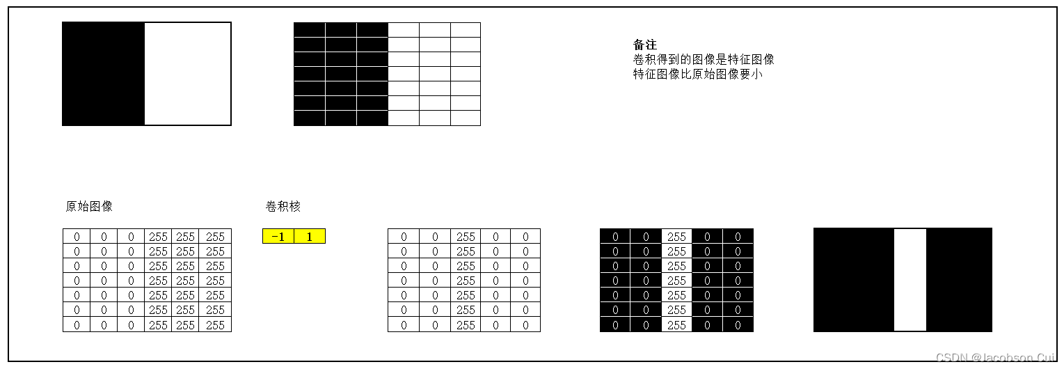
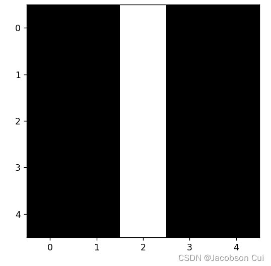
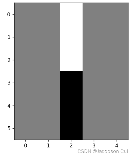
1. 图1使用卷积核 $\begin{pmatrix} 1&-1 \end{pmatrix}$ ，输出特征图

import torch
import matplotlib.pyplot as plt
import torch.nn.functional as F

picture = torch.Tensor([[0,0,0,255,255,255],
                      [0,0,0,255,255,255],
                      [0,0,0,255,255,255],
                      [0,0,0,255,255,255],
                      [0,0,0,255,255,255]])
#确定卷积网络
class GJ(torch.nn.Module):
    def __init__(self,kernel,kshape):
        super(GJ, self).__init__()
        kernel = torch.reshape(kernel,kshape)
        self.weight = torch.nn.Parameter(data=kernel, requires_grad=False)
    def forward(self, picture):
        picture = F.conv2d(picture,self.weight,stride=1,padding=0)
        return  picture
#确定卷积层
kernel = torch.tensor([-1.0,1.0])
#更改卷积层的形状适应卷积函数
kshape = (1,1,1,2)
#生成模型
model = GJ(kernel=kernel,kshape=kshape)
#更改图片的形状适应卷积层
picture = torch.reshape(picture,(1,1,5,6))
output = model(picture)
output = torch.reshape(output,(5,5))
plt.imshow(output,cmap='gray')
plt.show()

运行结果：

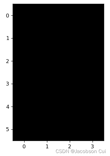
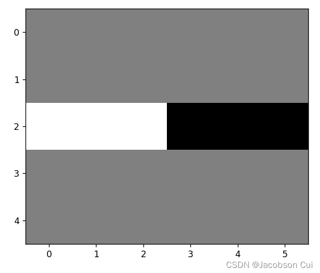
2. 图1使用卷积核 $\begin{pmatrix} 1 \\-1 \end{pmatrix}$ ，输出特征图

import torch
import matplotlib.pyplot as plt
import torch.nn.functional as F

picture = torch.Tensor([[0,0,0,255,255,255],
                      [0,0,0,255,255,255],
                      [0,0,0,255,255,255],
                      [0,0,0,255,255,255],
                      [0,0,0,255,255,255]])
#确定卷积网络
class GJ(torch.nn.Module):
    def __init__(self,kernel,kshape):
        super(GJ, self).__init__()
        kernel = torch.reshape(kernel,kshape)
        self.weight = torch.nn.Parameter(data=kernel, requires_grad=False)
    def forward(self, picture):
        picture = F.conv2d(picture,self.weight,stride=1,padding=0)
        return  picture
kernel = torch.tensor([-1.0,1.0])
#更改卷积和的形状为转置
kshape = (1,1,2,1)
model = GJ(kernel=kernel,kshape=kshape)
picture = torch.reshape(picture,(1,1,5,6))
output = model(picture)
output = torch.reshape(output,(6,4))
plt.imshow(output,cmap='gray')
plt.show()

运行结果：

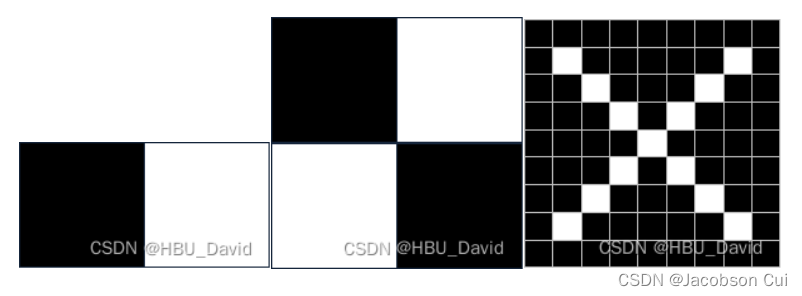
3. 图2使用卷积核 $\begin{pmatrix} 1&-1 \end{pmatrix}$ ，输出特征图

import torch
import matplotlib.pyplot as plt
import torch.nn.functional as F


#确定卷积网络
class GJ(torch.nn.Module):
    def __init__(self,kernel,kshape):
        super(GJ, self).__init__()
        kernel = torch.reshape(kernel,kshape)
        self.weight = torch.nn.Parameter(data=kernel, requires_grad=False)
    def forward(self, picture):
        picture = F.conv2d(picture,self.weight,stride=1,padding=0)
        return  picture


picture = torch.Tensor([[0,0,0,255,255,255],
                      [0,0,0,255,255,255],
                      [0,0,0,255,255,255],
                      [255,255,255,0,0,0],
                      [255,255,255,0,0,0],
                      [255,255,255,0,0,0]])
#确定卷积核
kernel = torch.tensor([-1.0,1.0])
kshape = (1,1,1,2)
#生成模型
model = GJ(kernel=kernel,kshape=kshape)
picture = torch.reshape(picture,(1,1,6,6))
print(picture)
output = model(picture)
output = torch.reshape(output,(6,5))
print(output)
plt.imshow(output,cmap='gray')
plt.show()

运行结果：

4. 图2使用卷积核 $\begin{pmatrix} 1\\-1 \end{pmatrix}$ ，输出特征图

import torch
import matplotlib.pyplot as plt
import torch.nn.functional as F


#确定卷积网络
class GJ(torch.nn.Module):
    def __init__(self,kernel,kshape):
        super(GJ, self).__init__()
        kernel = torch.reshape(kernel,kshape)
        self.weight = torch.nn.Parameter(data=kernel, requires_grad=False)
    def forward(self, picture):
        picture = F.conv2d(picture,self.weight,stride=1,padding=0)
        return  picture


picture = torch.Tensor([[0,0,0,255,255,255],
                      [0,0,0,255,255,255],
                      [0,0,0,255,255,255],
                      [255,255,255,0,0,0],
                      [255,255,255,0,0,0],
                      [255,255,255,0,0,0]])
kernel = torch.tensor([-1.0,1.0])
kshape = (1,1,2,1)
model = GJ(kernel=kernel,kshape=kshape)
picture = torch.reshape(picture,(1,1,6,6))
print(picture)
output = model(picture)
output = torch.reshape(output,(5,6))
print(output)
plt.imshow(output,cmap='gray')
plt.show()

运行结果：

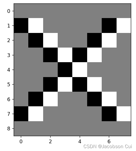
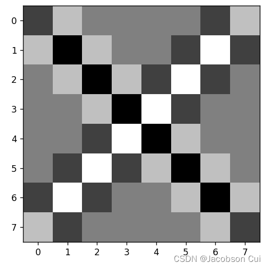
5. 图3使用卷积核 $\begin{pmatrix} 1 &-1 \end{pmatrix}$ ， $\begin{pmatrix} 1\\-1 \end{pmatrix}$ ， $\begin{pmatrix} 1 &-1 \\ -1&1 \end{pmatrix}$ ,输出特征图

import torch
import matplotlib.pyplot as plt
import torch.nn.functional as F


#确定卷积网络
class GJ(torch.nn.Module):
    def __init__(self,kernel,kshape):
        super(GJ, self).__init__()
        kernel = torch.reshape(kernel,kshape)
        self.weight = torch.nn.Parameter(data=kernel, requires_grad=False)
    def forward(self, picture):
        picture = F.conv2d(picture,self.weight,stride=1,padding=0)
        return  picture


picture = torch.Tensor(
                     [[255,255,255,255,255,255,255,255,255],
                      [255,0  ,255,255,255,255,255,0  ,255],
                      [255,255,0  ,255,255,255,0  ,255,255],
                      [255,255,255,0  ,255,0  ,255,255,255],
                      [255,255,255,255,0  ,255,255,255,255],
                      [255,255,255,0  ,255,0  ,255,255,255],
                      [255,255,0  ,255,255,255,0  ,255,255],
                      [255,0  ,255,255,255,255,255,0  ,255],
                      [255,255,255,255,255,255,255,255,255],])

#生成卷积核
kernel = torch.tensor([-1.0,1.0])
#更改卷积核的形状适应卷积函数
kshape = (1,1,1,2)
model = GJ(kernel=kernel,kshape=kshape)
picture = torch.reshape(picture,(1,1,9,9))
print(picture)
output = model(picture)
output = torch.reshape(output,(9,8))
print(output)
plt.imshow(output,cmap='gray')
plt.show()

运行结果：

import torch
import matplotlib.pyplot as plt
import torch.nn.functional as F


#确定卷积网络
class GJ(torch.nn.Module):
    def __init__(self,kernel,kshape):
        super(GJ, self).__init__()
        kernel = torch.reshape(kernel,kshape)
        self.weight = torch.nn.Parameter(data=kernel, requires_grad=False)
    def forward(self, picture):
        picture = F.conv2d(picture,self.weight,stride=1,padding=0)
        return  picture


picture = torch.Tensor(
                     [[255,255,255,255,255,255,255,255,255],
                      [255,0  ,255,255,255,255,255,0  ,255],
                      [255,255,0  ,255,255,255,0  ,255,255],
                      [255,255,255,0  ,255,0  ,255,255,255],
                      [255,255,255,255,0  ,255,255,255,255],
                      [255,255,255,0  ,255,0  ,255,255,255],
                      [255,255,0  ,255,255,255,0  ,255,255],
                      [255,0  ,255,255,255,255,255,0  ,255],
                      [255,255,255,255,255,255,255,255,255],])

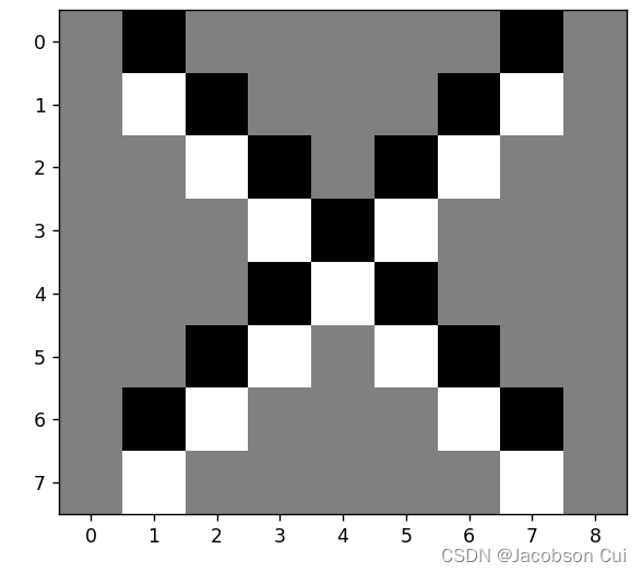
kernel = torch.tensor([-1.0,1.0])
kshape = (1,1,2,1)
model = GJ(kernel=kernel,kshape=kshape)
picture = torch.reshape(picture,(1,1,9,9))
print(picture)
output = model(picture)
output = torch.reshape(output,(8,9))
print(output)
plt.imshow(output,cmap='gray')
plt.show()

运行结果：

import torch
import matplotlib.pyplot as plt
import torch.nn.functional as F


#确定卷积网络
class GJ(torch.nn.Module):
    def __init__(self,kernel,kshape):
        super(GJ, self).__init__()
        kernel = torch.reshape(kernel,kshape)
        self.weight = torch.nn.Parameter(data=kernel, requires_grad=False)
    def forward(self, picture):
        picture = F.conv2d(picture,self.weight,stride=1,padding=0)
        return  picture


picture = torch.Tensor(
                     [[255,255,255,255,255,255,255,255,255],
                      [255,0  ,255,255,255,255,255,0  ,255],
                      [255,255,0  ,255,255,255,0  ,255,255],
                      [255,255,255,0  ,255,0  ,255,255,255],
                      [255,255,255,255,0  ,255,255,255,255],
                      [255,255,255,0  ,255,0  ,255,255,255],
                      [255,255,0  ,255,255,255,0  ,255,255],
                      [255,0  ,255,255,255,255,255,0  ,255],
                      [255,255,255,255,255,255,255,255,255],])

#确定卷积核
kernel = torch.tensor([[1.0,-1.0],
                       [-1.0,1.0]])
#更改卷积核的大小适配卷积函数
kshape = (1,1,2,2)
#生成网络模型
model = GJ(kernel=kernel,kshape=kshape)
picture = torch.reshape(picture,(1,1,9,9))
print(picture)
output = model(picture)
output = torch.reshape(output,(8,8))
print(output)
plt.imshow(output,cmap='gray')
plt.show()

运行结果：

作业2

卷积过程：

一、概念

卷积

连续型卷积的公式:

$s(x)=\int_{-\infty }^{\infty } f(\tau )g(x-\tau )d\tau$

离散型卷积的公式：

$s(x)=\sum_{\tau =-\infty }^{\infty } f(\tau )g(x-\tau )$

卷积的物理意义大概可以理解为：系统某一时刻的输出是由多个输入叠加的结果。

这里借用知乎大佬的形象描述：【深度学习之美25】卷积神经网络中“卷积”到底是个什么意思？

卷积核

卷积核即滤波器，其本质上是一个大小固定的数组，数组的标定点通常位于数组的中心。数组的大小被称为核支撑。单就技术而言，核支撑实际上仅仅由核数组的非零部分组成。

特征图

当图像像素值经过过滤器后得到的东西就是特征图。

特征选择

从原始特征中选择出一些最有效特征。

步长

步长即每次运算的时候卷积核移动的量。

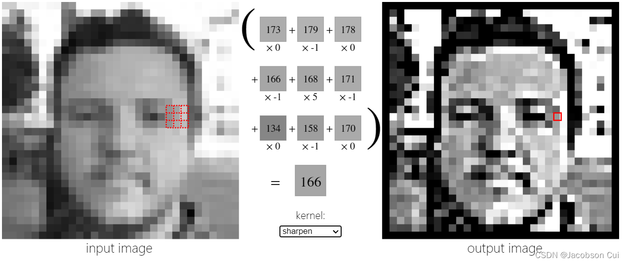
以上图为例，我们用橙色的矩阵（卷积核）在原始图像（绿色所示矩阵）上从左到右、从上到下滑动，每次滑动一个像素，滑动的距离就称为“步长”。在每个位置上，我们可以计算出两个矩阵间的相应元素乘积，并把点乘结果之和，存储在输出矩阵（粉色所示）中的每一个单元格中，这样就得到了特征图。

填充

填充也就是在矩阵的边界上填充一些值，以增加矩阵的大小，通常都用“0”来进行填充的。

感受野

感受野的定义是卷积神经网络每一层输出的特征图上的像素点在输入图片上映射的区域大小。即：特征图上的一个点对应输入图上的区域。

二、探究不同卷积核的作用

1、锐化

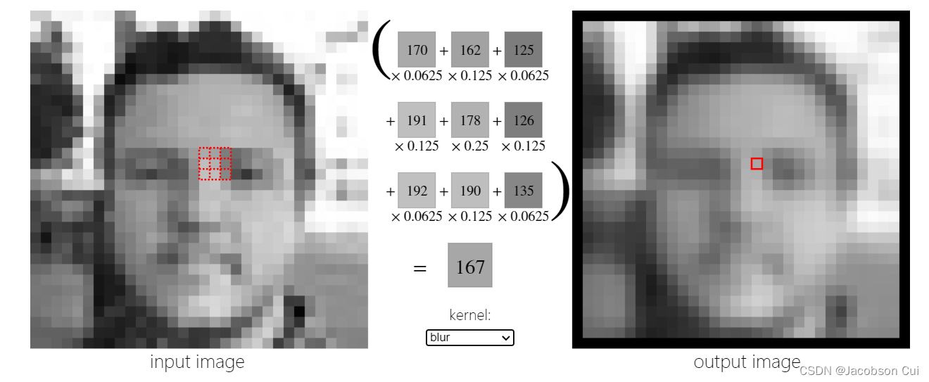
2、模糊

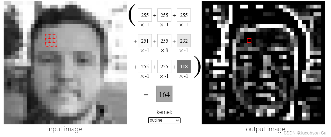
3、边缘检测

4、浮雕

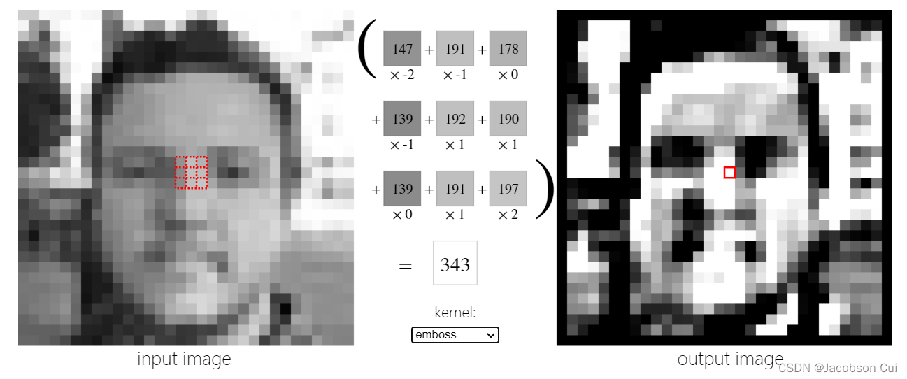
参考：Image Kernels explained visually (setosa.io)

三、编程实现

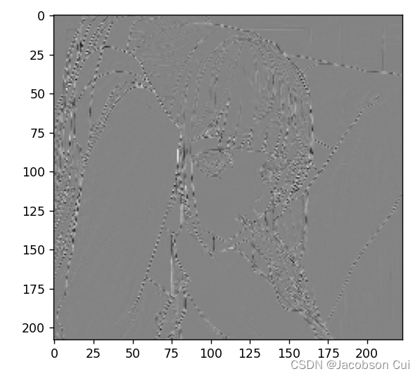
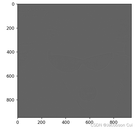
1、实现灰度图的边缘检测、锐化、模糊。（必做）

原图

边缘检测

import numpy as np
import torch
from torch import nn
from torch.autograd import Variable
from PIL import Image
import matplotlib.pyplot as plt

img = Image.open('2.jpg').convert('L') # 读入一张灰度图的图片
img = np.array(img, dtype='float32') # 将其转换为一个矩阵
plt.imshow(img.astype('uint8'), cmap='gray')
#使用Sobel算子进行边缘检测
im = torch.from_numpy(img.reshape((1, 1, img.shape[0], img.shape[1])))
conv1 = nn.Conv2d(1, 1, 3, bias=False) # 定义卷积

sobel_kernel = np.array([[-1, -1, -1], [-1, 8, -1], [-1, -1, -1]], dtype='float32') # 定义轮廓检测算子
sobel_kernel = sobel_kernel.reshape((1, 1, 3, 3)) # 适配卷积的输入输出
conv1.weight.data = torch.from_numpy(sobel_kernel) # 给卷积的 kernel 赋值

edge1 = conv1(Variable(im)) # 作用在图片上
edge1 = edge1.data.squeeze().numpy() # 将输出转换为图片的格式
plt.imshow(edge1, cmap='gray')
plt.show()

运行结果：

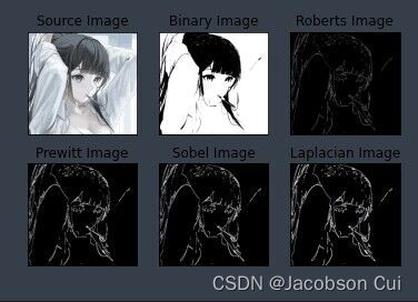
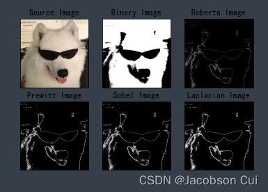
锐化

import cv2  
import numpy as np  
import matplotlib.pyplot as plt

#读取图像
img = cv2.imread('2.jpg')
lenna_img = cv2.cvtColor(img, cv2.COLOR_BGR2RGB)

#灰度化处理图像
grayImage = cv2.cvtColor(img, cv2.COLOR_BGR2GRAY)

#高斯滤波
gaussianBlur = cv2.GaussianBlur(grayImage, (3,3), 0)

#阈值处理
ret, binary = cv2.threshold(gaussianBlur, 127, 255, cv2.THRESH_BINARY)

#Roberts算子
kernelx = np.array([[-1,0],[0,1]], dtype=int)
kernely = np.array([[0,-1],[1,0]], dtype=int)
x = cv2.filter2D(binary, cv2.CV_16S, kernelx)
y = cv2.filter2D(binary, cv2.CV_16S, kernely)
absX = cv2.convertScaleAbs(x)     
absY = cv2.convertScaleAbs(y)    
Roberts = cv2.addWeighted(absX, 0.5, absY, 0.5, 0)

#Prewitt算子
kernelx = np.array([[1,1,1],[0,0,0],[-1,-1,-1]], dtype=int)
kernely = np.array([[-1,0,1],[-1,0,1],[-1,0,1]], dtype=int)
x = cv2.filter2D(binary, cv2.CV_16S, kernelx)
y = cv2.filter2D(binary, cv2.CV_16S, kernely)
absX = cv2.convertScaleAbs(x)  
absY = cv2.convertScaleAbs(y)    
Prewitt = cv2.addWeighted(absX,0.5,absY,0.5,0)

#Sobel算子
x = cv2.Sobel(binary, cv2.CV_16S, 1, 0)
y = cv2.Sobel(binary, cv2.CV_16S, 0, 1)    
absX = cv2.convertScaleAbs(x)   
absY = cv2.convertScaleAbs(y)    
Sobel = cv2.addWeighted(absX, 0.5, absY, 0.5, 0)

#拉普拉斯算法
dst = cv2.Laplacian(binary, cv2.CV_16S, ksize = 3)
Laplacian = cv2.convertScaleAbs(dst) 

#效果图
titles = ['Source Image', 'Binary Image', 'Roberts Image',
          'Prewitt Image','Sobel Image', 'Laplacian Image']  
images = [lenna_img, binary, Roberts, Prewitt, Sobel, Laplacian]  
for i in np.arange(6):  
    plt.subplot(2,3,i+1),plt.imshow(images[i],'gray')  
    plt.title(titles[i])  
    plt.xticks([]),plt.yticks([])  
plt.show()

运行结果：

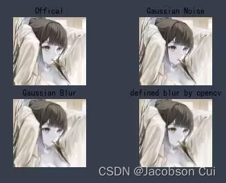
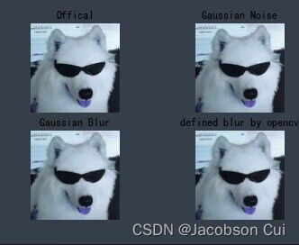
模糊

# 图像模糊处理
# 高斯模糊 gaussian blur
# 使用自编写高斯噪声及自编写高斯模糊函数与自带高斯函数作效果对比

import cv2
import numpy as np
import matplotlib.pyplot as plt


def clamp(pv):
    if pv > 255:
        return 255
    if pv < 0:
        return 0
    else:
        return pv


def gaussian_noise(image):        # 加高斯噪声
    h, w, c = image.shape
    for row in range(h):
        for col in range(w):
            s = np.random.normal(0, 20, 3)
            b = image[row, col, 0]   # blue
            g = image[row, col, 1]   # green
            r = image[row, col, 2]   # red
            image[row, col, 0] = clamp(b + s[0])
            image[row, col, 1] = clamp(g + s[1])
            image[row, col, 2] = clamp(r + s[2])
    dst = cv2.GaussianBlur(image, (15, 15), 0)  # 高斯模糊
    return dst, image


if __name__ == "__main__":
    src = cv2.imread('deer.jpeg')
    plt.subplot(2, 2, 1)
    plt.imshow(src)
    plt.axis('off')
    plt.title('Offical')

    output, noise = gaussian_noise(src)
    cvdst = cv2.GaussianBlur(src, (15, 15), 0)   # 高斯模糊

    plt.subplot(2, 2, 2)
    plt.imshow(noise)
    plt.axis('off')
    plt.title('Gaussian Noise')

    plt.subplot(2, 2, 3)
    plt.imshow(output)
    plt.axis('off')
    plt.title('Gaussian Blur')

    plt.subplot(2, 2, 4)
    plt.imshow(cvdst)
    plt.axis('off')
    plt.title('defined blur by opencv')

    plt.show()

运行结果：

2、调整卷积核参数，测试并总结。（必做）

以上述边缘检测为例，当增加步长时，图像的边界会变得模糊。

修改步长为4

conv1 = nn.Conv2d(2, 2, (3,3), stride=(4, 4),  bias=False) # 定义卷积

运行结果：

而增加padding后，图像提取的特征会更为全面，如设置padding为5

conv1 = nn.Conv2d(2, 2, (3,3), padding=5,  bias=False) # 定义卷积

运行结果：

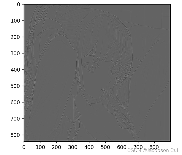
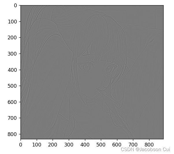
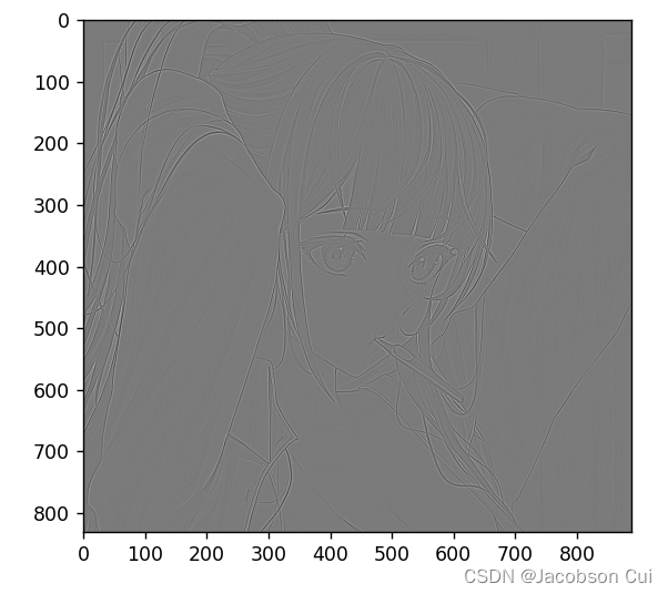
3、使用不同尺寸图片，测试并总结。（必做）

原图：

边缘检测

锐化

模糊

使用不同尺寸的图片，不会影响卷积的效果，但图像的特征对于卷积效果的影响却比较大，例如该图片的边缘检测效果就不如之前的图片清晰。

4、探索更多类型卷积核。（选做）

均值模糊：

    # （）内为一维卷积核，指在x，y方向偏移多少位
    dst1 = cv2.blur(image, (10, 1))

    # 此为中值模糊，常用于去除椒盐噪声
    dst2 = cv2.medianBlur(image, 10)

    # 自定义卷积核，执行模糊操作，也可定义执行锐化操作
    kernel = np.ones([5, 5], np.float32) / 25
    dst3 = cv2.filter2D(image, -1, kernel=kernel)

运动模糊：

    # 这里生成任意角度的运动模糊kernel的矩阵， degree越大，模糊程度越高
    M = cv2.getRotationMatrix2D((degree / 2, degree / 2), angle, 1)
    motion_blur_kernel = np.diag(np.ones(degree))
    motion_blur_kernel = cv2.warpAffine(motion_blur_kernel, M, (degree, degree))
    motion_blur_kernel = motion_blur_kernel / degree
    blurred = cv2.filter2D(image, -1, motion_blur_kernel)
    # convert to uint8
    cv2.normalize(blurred, blurred, 0, 255, cv2.NORM_MINMAX)

5、尝试彩色图片边缘检测。（选做）

import numpy as np
import torch
from torch import nn
from torch.autograd import Variable
from PIL import Image
import matplotlib.pyplot as plt

im = Image.open('2.jpg').convert('L') # 读入一张灰度图的图片
im = np.array(im, dtype='float32') # 将其转换为一个矩阵

# 可视化图片
plt.imshow(im.astype('uint8'), cmap='gray')
im = torch.from_numpy(im.reshape((1, 1, im.shape[0], im.shape[1])))
conv1 = nn.Conv2d(1,1, (3,3), bias=False) # 定义卷积

sobel_kernel = np.array([[-1, -1, -1], [-1, 8, -1], [-1, -1, -1]], dtype='float32') # 定义轮廓检测算子
sobel_kernel = sobel_kernel.reshape((1, 1, 3, 3)) # 适配卷积的输入输出
conv1.weight.data = torch.from_numpy(sobel_kernel) # 给卷积的 kernel 赋值

edge1 = conv1(Variable(im)) # 作用在图片上
edge1 = edge1.data.squeeze().numpy() # 将输出转换为图片的格式
plt.imshow(edge1, cmap='gray')

plt.show()

原图：

运行结果：

总结

这次作业了解了很多对图像进行卷积的操作尤其是对图像特征的提取，对于图像而言，每一幅图像都具有能够区别于其他类图像的自身特征，我们常常将某一类对象的多个或多种特性组合在一起，形成一个特征向量来代表该类对象，如果只有单个数值特征，则特征向量为一个一维向量，如果是n个特性的组合，则为一个n维特征向量。该类特征向量常常作为识别系统的输入。实际上，一个n维特征就是位于n维空间中的点，而识别分类的任务就是找到对这个n维空间的一种划分。