不同处理的土壤样本的各功能群落的香农指数（Shannon）和辛普森指数（Simpson）的计算（Python）

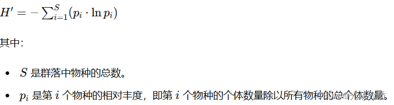
香农指数（Shannon Index）
香农指数（Shannon Index），也称为香农多样性指数（Shannon Diversity Index），是用来衡量群落中物种多样性的一种指数。它考虑了物种的丰富度（即物种数量）和均匀度（即各物种的相对丰度）。

 分析角度
- 如果所有物种的个体数量都非常均匀，则香农指数较高。
- 如果某个物种非常占优势，香农指数较低。
- 香农指数通常介于0到ln(S) 之间，其中  S 是物种总数。

辛普森指数（Simpson Index）

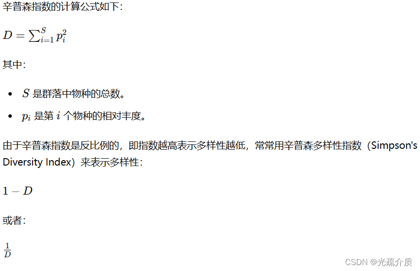
辛普森指数（Simpson Index）也是用来衡量群落多样性的指标，但它更侧重于描述物种的优势度。辛普森指数衡量的是在一个随机抽样中两个个体属于同一种类的概率。
辛普森指数的计算公式如下：

分析角度
- 如果群落中所有物种的个体数量都非常均匀，则辛普森多样性指数接近于0。
- 如果某个物种非常占优势，辛普森多样性指数接近于1。
- 辛普森指数可以用来衡量群落中物种的均匀度，指数越高表示均匀度越高。

Shannon更注重均匀度和物种的丰富度，是一个综合性较强的多样性指标。
Simpson更侧重于描述物种的优势度，对于衡量某些物种占优势的情况比较敏感。

数据结构如图

 

这里面我就根据需求直接定义了哪些Genus属于一类群落（例如：产甲烷群落等等） 

import pandas as pd
from scipy.stats import entropy
import numpy as np
import matplotlib.pyplot as plt

# 读取Excel文件
file_path = '/mnt/data/Genusbasic6.xlsx'
df = pd.read_excel(file_path)

# 定义各群落的Genus
methanogenic = ['Methanobacterium', 'Methanobrevibacter', 'Methanosaeta', 'Methanosarcina', 'Methanospirillum']
methane_oxidizing = ['Methylobacter', 'Methylomonas']
iron_reducing = ['Geobacter', 'Shewanella', 'Thiobacillus']
sulfate_reducing = ['Desulfobulbus', 'Desulfotomaculum', 'Desulfovibrio']

# 定义计算多样性指数的函数
def calculate_diversity(df, group_columns):
    diversity_indices = []
    for group in df['Group'].unique():
        group_data = df[df['Group'] == group]
        for name, columns in group_columns.items():
            group_counts = group_data[columns].values.flatten()
            group_counts = group_counts[group_counts > 0]  # 移除零计数以进行多样性计算
            if len(group_counts) > 0:
                shannon_index = entropy(group_counts)
                simpson_index = 1 - sum((group_counts / sum(group_counts))**2)
            else:
                shannon_index = np.nan
                simpson_index = np.nan
            diversity_indices.append({
                'Group': group,
                'Community': name,
                'Shannon Index': shannon_index,
                'Simpson Index': simpson_index
            })
    return pd.DataFrame(diversity_indices)

# 定义群落分类
group_columns_corrected = {
    'Methanogenic': methanogenic,
    'Methane Oxidizing': methane_oxidizing,
    'Iron Reducing': iron_reducing,
    'Sulfate Reducing': sulfate_reducing
}

# 计算多样性指数
diversity_df_corrected = calculate_diversity(df, group_columns_corrected)

# 绘制多样性指数图的函数
def plot_diversity_indices(df, index_name):
    communities = df['Community'].unique()
    groups = df['Group'].unique()
    
    for community in communities:
        plt.figure(figsize=(10, 6))
        community_data = df[df['Community'] == community]
        plt.bar(community_data['Group'], community_data[index_name])
        plt.xlabel('Group')
        plt.ylabel(index_name)
        plt.title(f'{index_name} for {community} Community')
        plt.xticks(rotation=45)
        plt.show()

# 绘制香农指数图
plot_diversity_indices(diversity_df_corrected, 'Shannon Index')

# 绘制辛普森指数图
plot_diversity_indices(diversity_df_corrected, 'Simpson Index')

最后得到数据

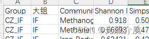
这里面我加了大组分类，是想直接粗略看一下处理的影响

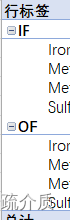
然后数据透视表就可以看到各处理下各分组的值的对比啦