机器学习与数据挖掘实验2-使用梯度下降法训练多远线性回归模型

 

import numpy as np
import pandas as pd
from matplotlib import pyplot as plt
from mpl_toolkits.mplot3d import Axes3D
from sklearn.model_selection import train_test_split

train_data = pd.read_csv("E:\\Downloads\\PyCharm 2022.3.2\\pythonProject\\data2.txt", header=1,
                         names=['Size', 'Bedrooms', 'Price'])
x = np.array(train_data, 'float32')
x = np.delete(x, [2], axis=1)
y = np.array(train_data.Price, 'float32')

x_train, x_test, y_train, y_test = train_test_split(x, y, test_size=0.2, random_state=0)


def scaler(train, test):

    min = train.min(axis=0)
    max = train.max(axis=0)
    gap = max - min
    train -= min
    train /= gap
    test -= min
    test /= gap
    return train, test


def min_max_gap(train):

    min = train.min(axis=0)
    max = train.max(axis=0)
    gap = max - min
    return min, max, gap


y_min, y_max, y_gap = min_max_gap(y_train)
x_train_origin = x_train.copy()


def loss_function(x, y, W):

    y_hat = x.dot(W.T)
    loss = y_hat - y.reshape((len(y_hat), 1))
    cost = np.sum(loss ** 2) / (2 * len(x))
    return cost


x_train, x_test = scaler(x_train, x_test)
y_train, y_test = scaler(y_train, y_test)

iterations = 1000
alpha = 0.1
weight = np.array([[1, 1], ])


# print(loss_function(x_train, y_train, weight))


def gradient_descent(x, y, w, lr, iterations):

    l_history = np.zeros(iterations)
    w_history = np.zeros((iterations, 2))
    for iter in range(iterations):
        y_hat = x.dot(w.T)
        loss = y_hat - y.reshape((len(y_hat), 1))
        derivative_w = x.T.dot(loss) / len(x)
        derivative_w = derivative_w.T
        w = w - lr * derivative_w
        l_history[iter] = loss_function(x, y, w)
        w_history[iter] = w
    return l_history, w_history


def liner_regression(x, y, weight, alpha, iter):
    loss_history, weight_history = gradient_descent(x, y, weight, alpha, iter)
    print("训练最终损失", loss_history[-1])
    return loss_history, weight_history


loss_history, weight_history = liner_regression(x_train, y_train, weight, alpha, iterations)
print(weight_history)
print("#" * 20)
print(loss_history)

plt.rcParams["font.sans-serif"] = ["SimHei"]
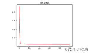
plt.title("损失函数图")
plt.plot(np.arange(iterations), loss_history, 'r')
plt.show()

theat = weight_history[-1]
print(theat)

x1 = np.linspace(x_train[:, 0].min(), x_train[:, 0].max(), 100)
x2 = np.linspace(x_train[:, 1].min(), x_train[:, 1].max(), 100)
x1, x2 = np.meshgrid(x1, x2)
f = theat[0] * x1 + theat[1] * x2

fig = plt.figure()
Ax = fig.add_axes(Axes3D(fig))
Ax.plot_surface(x1, x2, f,
                rstride=1,
                cstride=1,
                cmap=plt.get_cmap('winter'))

plt.title("3D散点图")
Ax.scatter(x_train[:, 0], x_train[:, 1], y_train, c="r")


def costs_fun(theat1, theat2):
    global x_train, y_train
    theat = np.array([theat1, theat2])
    y_hat = x_train.dot(theat.T)
    loss = y_hat.reshape(len(y_hat), 1)
    cost = np.sum(loss * 2) / (2 * len(x_train))
    return cost


theat1 = np.arange(0.0, 1.0, 0.005)
theat2 = np.arange(0.0, 1.0, 0.005)
theat1, theat2 = np.meshgrid(theat1, theat2)
f = np.array(list(map(lambda t: costs_fun(t[0], t[1]), zip(theat1.flatten(), theat2.flatten()))))
f = f.reshape(theat1.shape[0], -1)
fig = plt.figure()
Ax = fig.add_axes(Axes3D(fig))
Ax.plot_surface(theat1, theat2, f, rstride=1, cstride=1, cmap=plt.get_cmap('winter'))
plt.title('在theat1 theat2两个参数下损失变化图')
plt.show()

x_plan = np.random.randn(1650, 2)
x_train, x_plan = scaler(x_train_origin, x_plan)

n = weight_history.shape[0] - 1
t = weight_history[n, :].reshape(2, -1)
y_plan = np.dot(x_plan, t)

y_value = y_plan * y_gap + y_min

print(x_plan)
print(y_value)
print("预测值", y_value.astype(int))

最终得到的损失函数图：

数据散点图：

损失变化图：

最终的数据散点图与损失变化图的3D图像无法呈现的问题：本电脑上装的matplotlib 3.6.2不能够显示3D图像，而3.4.3版本的可以，因此可以选择将该包的版本更换。另一种解决方法是将代码Ax = Axes3D(fig) 改为 Ax = fig.add_axes(Axes3D(fig))，也可以解决这个问题。