机器学习与数据挖掘实验3-求解对数几率回归问题

 

import numpy as np
import matplotlib.pyplot as plt
import matplotlib as mpl
from sklearn.metrics import accuracy_score
def loaddata():
    data = np.loadtxt('E:\\Downloads\\PyCharm 2022.3.2\\pythonProject\\data1.txt',delimiter=',')
    n = data.shape[1] - 1  # 特征数
    X = data[:, 0:n]
    y = data[:, -1].reshape(-1, 1)
    return X, y
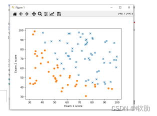
def plot(X,y):
    pos = np.where(y==1)
    neg = np.where(y==0)
    plt.scatter(X[pos[0],0],X[pos[0],1],marker='x')
    plt.scatter(X[neg[0], 0], X[neg[0], 1], marker='o')
    plt.xlabel('Exam 1 score')
    plt.ylabel('Exam 2 score')
    plt.show()
X,y = loaddata()
plot(X,y)

def sigmoid(z):
    r = 1/(1+np.exp(-z))
    return r
def hypothesis(X,theta):
    z=np.dot(X,theta)
    return sigmoid(z)
def computeCost(X,y,theta):
    m = X.shape[0]
#补充计算代价的代码；
    z = -1 * y * np.log(hypothesis(X, theta)) - (1 - y) * np.log(1 - hypothesis(X, theta))

    return np.sum(z)/m
# 梯度下降函数

def gradientDescent(X, y, theta, iterations, alpha):
    m = X.shape[0]
    X = np.hstack((np.ones((m, 1)), X))
    for i in range(iterations):
        for j in range(len(theta)):
            theta_temp[j] = theta_temp[j] - (alpha / m) * np.sum((hypothesis(X, theta) - y) * X[:,j].reshape(-1,1))
        theta = theta_temp
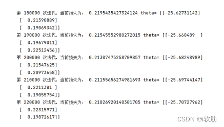
        if (i % 10000 == 0):
            print('第', i, '次迭代，当前损失为：', computeCost(X, y, theta), 'theta=', theta)
    return theta

def predict(X):
    # 在x最前面插入全1的列
    c = np.ones(X.shape[0]).transpose()
    X = np.insert(X, 0, values=c, axis=1)
    #求解假设函数的值
    h = hypothesis(X,theta)
    #根据概率值决定最终的分类,>=0.5为1类，<0.5为0类
    h[h>=0.5]=1
    h[h<0.5]=0
    return h

X,y = loaddata()
n = X.shape[1]#特征数
theta = np.zeros(n+1).reshape(n+1, 1)
# theta是列向量,+1是因为求梯度时X前会增加一个全1列
theta_temp = np.zeros(n+1).reshape(n+1, 1)
iterations = 250000
alpha = 0.008

theta = gradientDescent(X,y,theta,iterations,alpha)
print('theta=\n',theta)

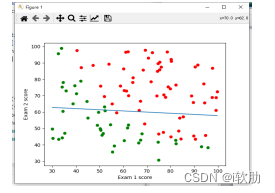
def plotDescisionBoundary(X,y,theta):
    cm_dark = mpl.colors.ListedColormap(['g', 'r'])
    plt.xlabel('Exam 1 score')
    plt.ylabel('Exam 2 score')
    plt.scatter(X[:,0],X[:,1],c=np.array(y).squeeze(),cmap=cm_dark,s=30)
    x1 = np.arange(min(X[:, 0]), max(X[:, 0]), 0.1)
    x2 = -(theta[1] * x1 + theta[0] / theta[2])

    plt.plot(x1,x2)
    plt.show()

plotDescisionBoundary(X,y,theta)

最终得到的数据散点图：

决策边界：

迭代损失值：