吴恩达机器学习课后作业ex2（python实现）

糖醋web排骨

已于 2022-11-21 12:52:05 修改

阅读量1.1k

点赞数 3

文章标签： python 开发语言

于 2022-11-20 20:06:20 首次发布

本文链接：https://blog.csdn.net/weixin_55037029/article/details/127953119

版权

ex2分为两个部分，第一个部分为线性的逻辑回归，第二部分则是非线性。

第一部分

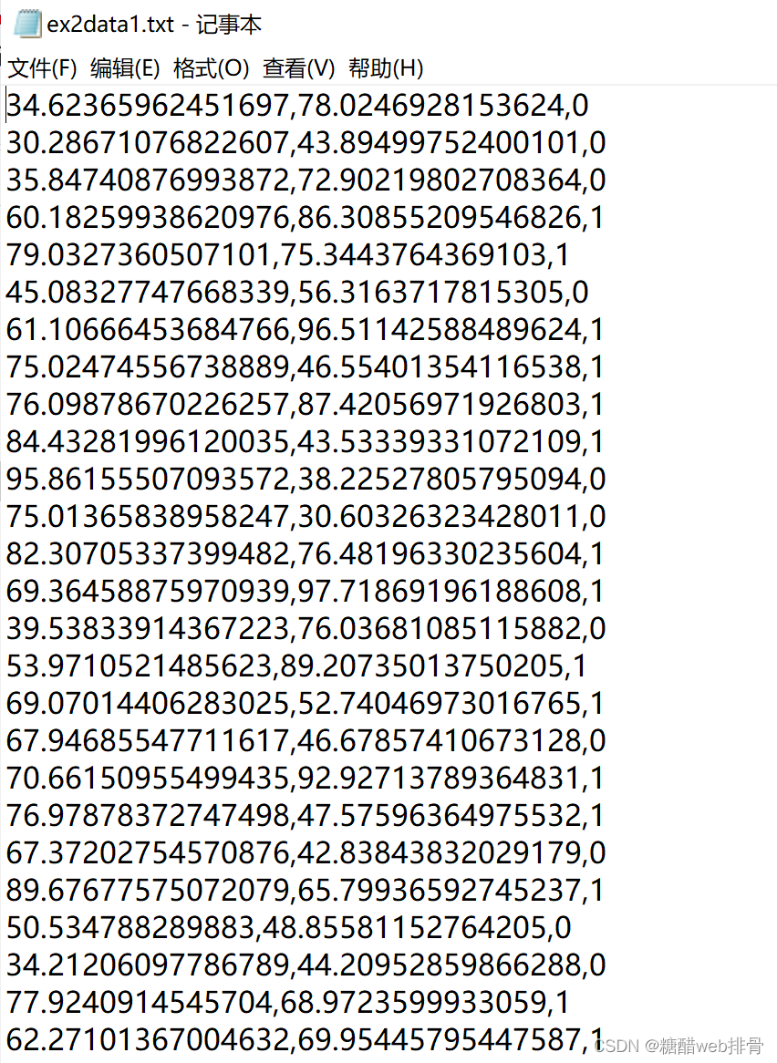
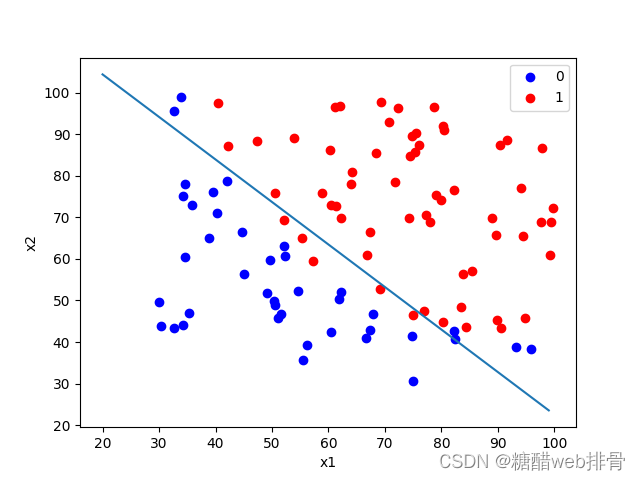
数据集：

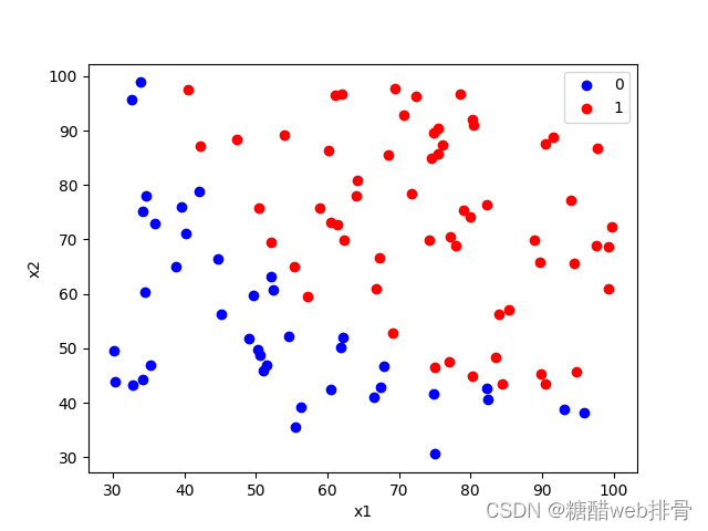
将图像画出来：

import pandas as pd
import numpy as np
import matplotlib.pyplot as plt


# 读取数据
df = pd.read_csv('ex2data1.txt', names=['x1', 'x2', 'y'])
df0 = df[df['y'] == 0]
df1 = df[df['y'] == 1]
# 画散点图
plt.scatter(df0.iloc[:, 0], df0.iloc[:, 1], c='b')
plt.scatter(df1.iloc[:, 0], df1.iloc[:, 1], c='r')
plt.xlabel('x1')
plt.ylabel('x2')
plt.legend('01')
plt.show()

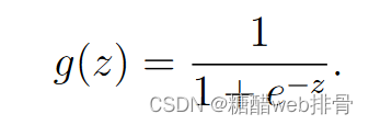
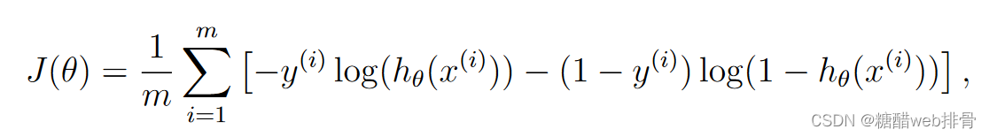
sigmoid函数为：

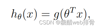
预测函数h(x)为：

代码实现：

def g(z):
    return 1 / (1 + np.exp(-z))


def h(theta, x):
    return g(np.dot(x, theta))

Cost function：

def cost(theta, x, y):
    theta = np.matrix(theta)
    left = np.multiply(-y, np.log(g(x*theta)))
    right = np.multiply((1-y), np.log(1-g(x*theta)))
    return np.sum(left-right)/(len(x))

下降梯度：

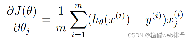
这里我先手动实现了梯度下降：

a = 0.01
for i in range(200000):
    error = g(x * theta) - y
    for i in range(3):
        term = np.multiply(error, x[:, i])
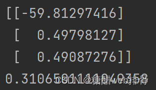
        theta[i, 0] -= a * np.sum(term) / len(x)

经过200000次迭代，效果才比较好：

此时的theta和损失值为：

第一种方法源码：

import pandas as pd
import numpy as np
import matplotlib.pyplot as plt


# 读取数据
df = pd.read_csv('ex2data1.txt', names=['x1', 'x2', 'y'])
df0 = df[df['y'] == 0]
df1 = df[df['y'] == 1]
# 画散点图
plt.scatter(df0.iloc[:, 0], df0.iloc[:, 1], c='b')
plt.scatter(df1.iloc[:, 0], df1.iloc[:, 1], c='r')
plt.xlabel('x1')
plt.ylabel('x2')
plt.legend('01')
plt.show()


theta = np.matrix(np.zeros((3, 1)))
x = np.matrix(df.iloc[:, [0, 1]])
y = np.matrix(df.iloc[:, 2]).T
x = np.insert(x, 0, np.ones(len(x)), axis=1)


def g(z):
    return 1 / (1 + np.exp(-z))


def h(theta, x):
    return g(np.dot(x, theta))


def cost(theta, x, y):
    theta = np.matrix(theta)
    left = np.multiply(-y, np.log(g(x*theta)))
    right = np.multiply((1-y), np.log(1-g(x*theta)))
    return np.sum(left-right)/(len(x))


a = 0.01
for i in range(200000):
    error = g(x * theta) - y
    for i in range(3):
        term = np.multiply(error, x[:, i])
        theta[i, 0] -= a * np.sum(term) / len(x)

print(theta)
print(cost(theta, x, y))
px = [i for i in range(20, 100)]
py = [-(px[i] * theta[1, 0] + theta[0, 0]) / theta[2, 0] for i in range(len(px))]

plt.scatter(df0.iloc[:, 0], df0.iloc[:, 1], c='b')
plt.scatter(df1.iloc[:, 0], df1.iloc[:, 1], c='r')
plt.plot(px, py)
plt.xlabel('x1')
plt.ylabel('x2')
plt.legend('01')
plt.show()

还有另一种方法进行梯度下降，就是用scipy.optimize优化器来进行最优参数拟合，其余部分与第一种方法类似，多定义一个梯度下降函数，将梯度下降部分改为：

def gradient(theta, X, y):
    theta = np.matrix(theta).T
    X = np.matrix(X)
    y = np.matrix(y)

    grad = np.zeros((3, 1))

    error = g(X * theta) - y

    for i in range(3):
        term = np.multiply(error, X[:, i])
        grad[i, 0] = np.sum(term) / len(X)

    return grad


result = opt.fmin_tnc(func=cost, x0=theta, fprime=gradient, args=(x, y))
theta = result[0]

拟合效果非常不错：

此时的theta与损失值为：

比第一种方法简直好太多。

第二种方法源码：

import pandas as pd
import numpy as np
import matplotlib.pyplot as plt
import scipy.optimize as opt


# 读取数据
df = pd.read_csv('ex2data1.txt', names=['x1', 'x2', 'y'])
df0 = df[df['y'] == 0]
df1 = df[df['y'] == 1]
# 初始化参数
theta = np.matrix(np.zeros((3, 1)))
x = np.matrix(df.iloc[:, [0, 1]])
y = np.matrix(df.iloc[:, 2]).T
x = np.insert(x, 0, np.ones(len(x)), axis=1)


def g(z):
    return 1 / (1 + np.exp(-z))


def h(theta, x):
    return g(np.dot(x, theta))


def cost(theta, x, y):
    theta = np.matrix(theta).T
    left = np.multiply(-y, np.log(g(x*theta)))
    right = np.multiply((1-y), np.log(1-g(x*theta)))
    return np.sum(left-right)/(len(x))


def gradient(theta, X, y):
    theta = np.matrix(theta).T
    X = np.matrix(X)
    y = np.matrix(y)

    grad = np.zeros((3, 1))

    error = g(X * theta) - y

    for i in range(3):
        term = np.multiply(error, X[:, i])
        grad[i, 0] = np.sum(term) / len(X)

    return grad


result = opt.fmin_tnc(func=cost, x0=theta, fprime=gradient, args=(x, y))
theta = result[0]
print(theta)
print(cost(theta, x, y))
px = [i for i in range(20, 100)]
py = [-(px[i] * theta[1] + theta[0]) / theta[2] for i in range(len(px))]

plt.scatter(df0.iloc[:, 0], df0.iloc[:, 1], c='b')
plt.scatter(df1.iloc[:, 0], df1.iloc[:, 1], c='r')
plt.plot(px, py)
plt.xlabel('x1')
plt.ylabel('x2')
plt.legend('01')
plt.show()

第二部分

数据集：

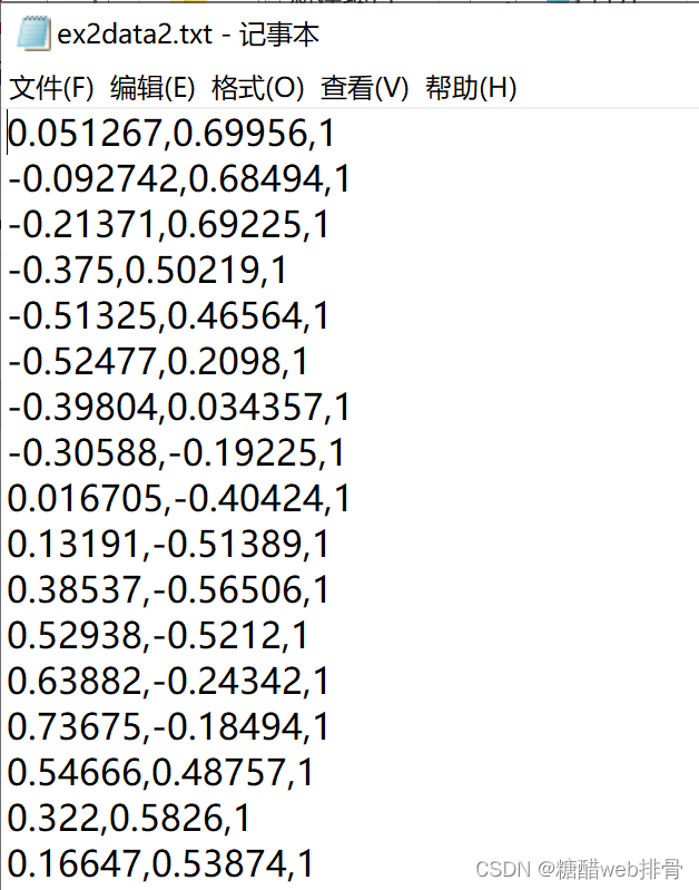
将其画为散点图展示：

import pandas as pd
import matplotlib.pyplot as plt
import numpy as np


# 读取数据
df = pd.read_csv('ex2data2.txt', names=['x1', 'x2', 'y'])
df0 = df[df['y'] == 0]
df1 = df[df['y'] == 1]
# 画散点图
plt.scatter(df0.iloc[:, 0], df0.iloc[:, 1], c='b')
plt.scatter(df1.iloc[:, 0], df1.iloc[:, 1], c='r')
plt.xlabel('x1')
plt.ylabel('x2')
plt.legend('01')
plt.show()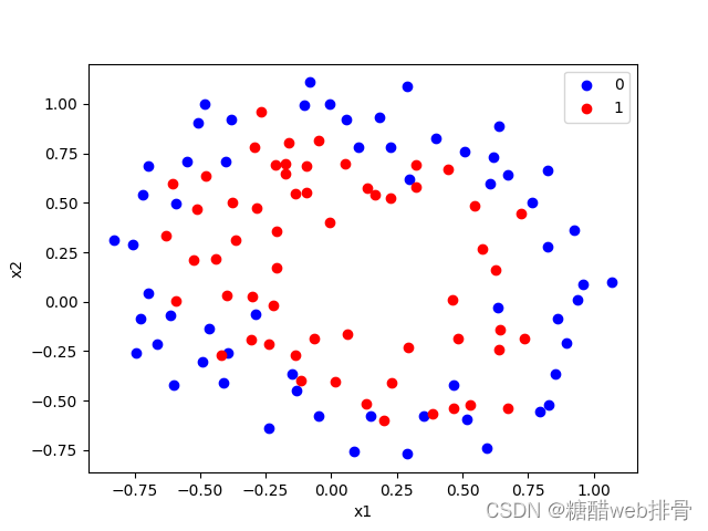

这里很明显是非线性的关系，查看说明文档发现需要构造特征为：

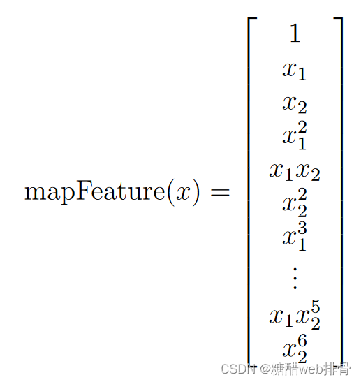
# 构造x
x = df.iloc[:, [0, 1]]
x1 = df.iloc[:, 0]
x2 = df.iloc[:, 1]
degree = 6
for i in range(1, degree+1):
    for j in range(0, i+1):
        x['F' + str(i-j) + str(j)] = np.power(x1, i-j) * np.power(x2, j)

x.drop('x1', axis=1, inplace=True)
x.drop('x2', axis=1, inplace=True)
x = np.matrix(x)
x = np.insert(x, 0, np.ones(len(x)), axis=1)

然后和第一问一样，实现函数，但是注意这里的cost function要添加正则化项：

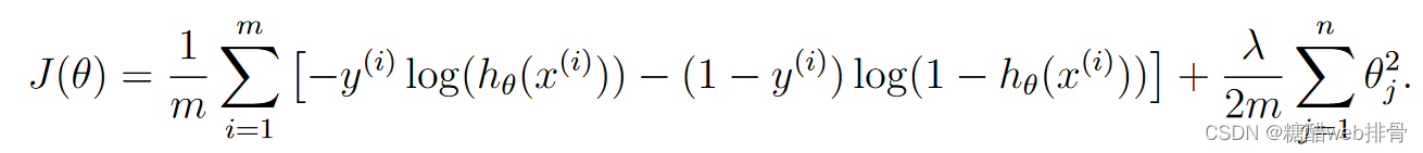
def cost(theta, x, y):
    theta = np.matrix(theta)
    first = -np.multiply(y, np.log(h(theta, x)))
    second = -np.multiply((1-y), np.log(1 - h(theta, x)))
    third = sita * np.sum(np.power(theta, 2)) / len(theta)
    return np.sum(first + second) / len(x) + third

使用优化器进行优化求最优解（ $\lambda =0.001$ ）：

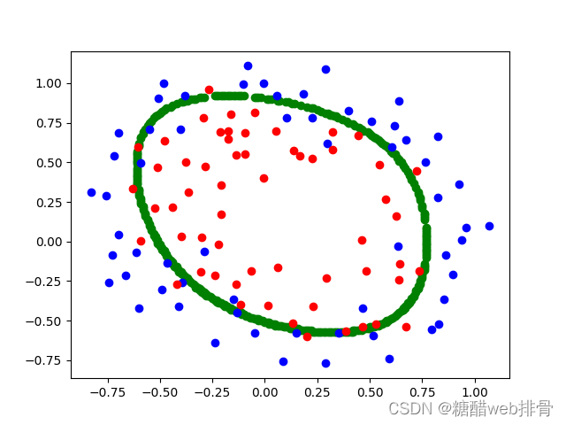
此时的cost为0.45801011485103144。进一步调低 $\lambda =0$ ，此时结果为：

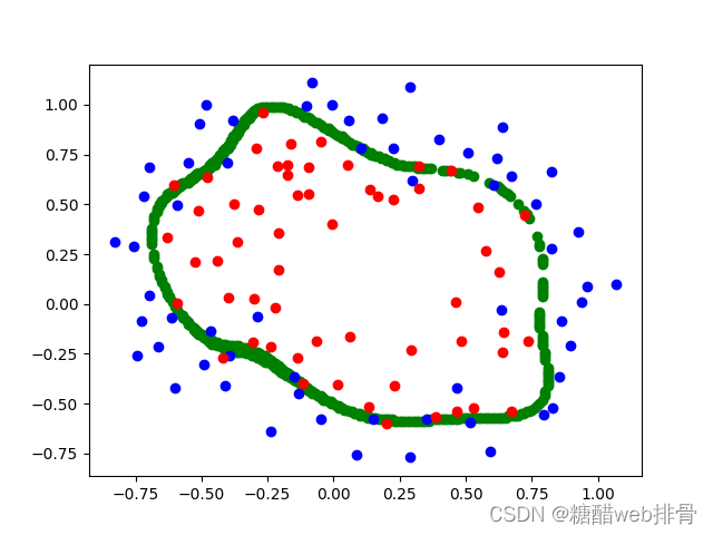
cost为0.26097691012426083。

源码：

import pandas as pd
import matplotlib.pyplot as plt
import numpy as np
import scipy.optimize as opt


# 读取数据
df = pd.read_csv('ex2data2.txt', names=['x1', 'x2', 'y'])
df0 = df[df['y'] == 0]
df1 = df[df['y'] == 1]
# 画散点图
plt.scatter(df0.iloc[:, 0], df0.iloc[:, 1], c='b')
plt.scatter(df1.iloc[:, 0], df1.iloc[:, 1], c='r')
plt.xlabel('x1')
plt.ylabel('x2')
plt.legend('01')
plt.show()

# 构造x
x = df.iloc[:, [0, 1]]
x1 = df.iloc[:, 0]
x2 = df.iloc[:, 1]
degree = 6
for i in range(1, degree+1):
    for j in range(0, i+1):
        x['F' + str(i-j) + str(j)] = np.power(x1, i-j) * np.power(x2, j)

x.drop('x1', axis=1, inplace=True)
x.drop('x2', axis=1, inplace=True)
x = np.matrix(x)
x = np.insert(x, 0, np.ones(len(x)), axis=1)

# 构造y
y = np.matrix(df.iloc[:, 2]).T

# 构造theta
theta = np.zeros(x.shape[1])
sita = 0


# g(z)
def g(z):
    return 1 / (1 + np.exp(-z))


# h(x):
def h(theta, x):
    return g(np.dot(x, theta.T))


def cost(theta, x, y):
    theta = np.matrix(theta)
    first = -np.multiply(y, np.log(h(theta, x)))
    second = -np.multiply((1-y), np.log(1 - h(theta, x)))
    third = sita * np.sum(np.power(theta, 2)) / len(theta)
    return np.sum(first + second) / len(x) + third


print(cost(theta, x, y))


def gradient(theta, X, y):
    theta = np.matrix(theta).T
    X = np.matrix(X)
    y = np.matrix(y)
    grad = np.zeros((28, 1))

    error = g(X * theta) - y

    for i in range(28):
        term = np.multiply(error, X[:, i])
        if i == 0:
            grad[i, 0] = np.sum(term) / len(X)
        else:
            grad[i, 0] = np.sum(term) / len(X) + sita * theta[i, 0] / len(X)

    return grad


result = opt.fmin_tnc(func=cost, x0=theta, fprime=gradient, args=(x, y))
theta = result[0]
print(theta)
print(cost(theta, x, y))

x1 = np.arange(-1, 1, 0.01)
x2 = np.arange(-1, 1, 0.01)
temp = []
for i in range(len(x1)):
    for j in range(len(x2)):
        temp.append([x1[i], x2[j]])
temp = pd.DataFrame(temp)
x1 = temp.iloc[:, 0]
x2 = temp.iloc[:, 1]
xx = pd.DataFrame()
for i in range(1, degree+1):
    for j in range(0, i+1):
        xx['F' + str(i-j) + str(j)] = np.power(x1, i-j) * np.power(x2, j)

xx = np.matrix(xx)
xx = np.insert(xx, 0, np.ones(len(xx)), axis=1)
theta = np.matrix(theta).T
res = np.dot(xx, theta)
res = g(res)

px = []
x1 = np.arange(-1, 1, 0.01)
x2 = np.arange(-1, 1, 0.01)
for i in range(len(res)):
    if abs(res[i, 0] - 0.5) < 0.04:
        px.append([xx[i, 1], xx[i, 2]])

print(len(px))
for i in range(len(px)):
    plt.scatter(px[i][0], px[i][1], c='g')
plt.scatter(df0.iloc[:, 0], df0.iloc[:, 1], c='b')
plt.scatter(df1.iloc[:, 0], df1.iloc[:, 1], c='r')
plt.show()