Kaggle房价预测问题

1 所提供的数据集

• train.csv - the training set
• test.csv - the test set
• data_description.txt - full description of each column, originally prepared by Dean De Cock but lightly edited to match the column names used here
• sample_submission.csv - a benchmark submission from a linear regression on year and month of sale, lot square footage, and number of bedrooms

2 房价预测

2.1 检视数据集

查看一下数据集是什么样子的。
导入相关库。

import numpy as np
import pandas as pd

导入数据集。

train_df = pd.read_csv('./train.csv', index_col = 0)
test_df = pd.read_csv('./test.csv', index_col = 0)

数据集有79种特征。

2.2 合并数据

为啥了使得数据预处理更为方便，我们将数据转换为正态分布性数据。

%matplotlib inline
prices = pd.DataFrame({"price":train_df["SalePrice"], "log(price + 1)":np.log1p(train_df["SalePrice"])})
prices.hist()

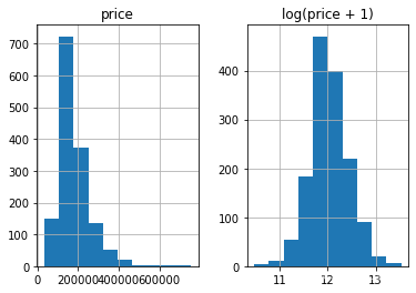
y_train = np.log1p(train_df.pop('SalePrice'))
all_df = pd.concat((train_df, test_df), axis = 0)

2.3 变量转换

all_df['MSSubClass'] = all_df['MSSubClass'].astype(str)
all_dummy_df = pd.get_dummies(all_df)
all_dummy_df.head()

处理缺失值。这里使用平均值来填充缺失值。

mean_cols = all_dummy_df.mean()
all_dummy_df = all_dummy_df.fillna(mean_cols)
numeric_cols = all_df.columns[all_df.dtypes != 'object']

计算标准分布：(X-X’)/s

让我们的数据点更平滑，更便于计算。

注意：我们这里也是可以继续使用Log的，我只是给大家展示一下多种“使数据平滑”的办法。

numeric_col_means = all_dummy_df.loc[:, numeric_cols].mean()
numeric_col_std = all_dummy_df.loc[:, numeric_cols].std()
all_dummy_df.loc[:, numeric_cols] = (all_dummy_df.loc[:, numeric_cols] - numeric_col_means) / numeric_col_std

2.4 建立模型

dummy_train_df = all_dummy_df.loc[train_df.index]
dummy_test_df = all_dummy_df.loc[test_df.index]

岭回归模型

from sklearn.linear_model import Ridge
from sklearn.model_selection import cross_val_score
# 将DF转化为NumPy Array
X_train = dummy_train_df.values
X_test = dummy_test_df.values

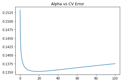
绘制学习曲线。

alphas = np.logspace(-3, 2, 50)
test_scores = []
for alpha in alphas:
    clf = Ridge(alpha)
    test_score = np.sqrt(-cross_val_score(clf, X_train, y_train, cv = 10, scoring="neg_mean_squared_error"))
    test_scores.append(np.mean(test_score))

import matplotlib.pyplot as plt
%matplotlib inline
plt.plot(alphas, test_scores)
plt.title("Alpha vs CV Error")

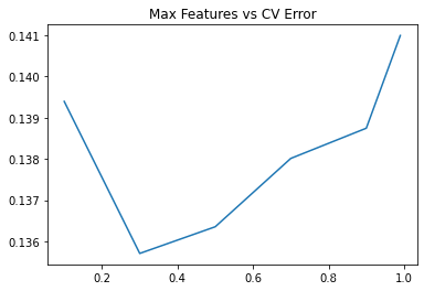
随机森林模型

from sklearn.ensemble import RandomForestRegressor

绘制学习曲线。

max_features =[.1, .3, .5, .7, .9, .99]
test_scores = []
for max_feat in max_features:
    clf = RandomForestRegressor(n_estimators=200, max_features=max_feat)
    test_score = np.sqrt(-cross_val_score(clf, X_train, y_train, cv = 10, scoring="neg_mean_squared_error"))
    test_scores.append(np.mean(test_score))
    
plt.plot(max_features, test_scores)
plt.title("Max Features vs CV Error")

模型合体

ridge = Ridge(alpha = 15)
rf  = RandomForestRegressor(n_estimators=300, max_features=.3)

ridge.fit(X_train,y_train)
rf.fit(X_train,y_train)

y_ridge = np.expm1(ridge.predict(X_test))
y_rf = np.expm1(rf.predict(X_test))

y_final = (y_ridge + y_rf) / 2

2.6 保存结果

outputpath='C:/Users/LENOVO/Desktop/submission.csv'
submission_df.to_csv(outputpath,sep=',',index=False,header=False)

3 模型进阶,高级Ensemble

Bagging

Bagging把很多的小分类器放在一起，每个train随机的一部分数据，然后把它们的最终结果综合起来（多数投票制）。

Sklearn已经直接提供了这套构架，我们直接调用就行：

from sklearn.linear_model import Ridge
ridge = Ridge(15)

from sklearn.ensemble import BaggingRegressor
from sklearn.model_selection import cross_val_score

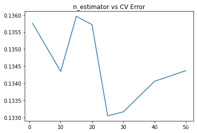
在这里，我们用CV结果来测试不同的分类器个数对最后结果的影响。

注意，我们在部署Bagging的时候，要把它的函数base_estimator里填上你的小分类器（ridge）

params = [1, 10, 15, 20, 25, 30, 40, 50]
test_scores = []
for param in params:
    clf = BaggingRegressor(n_estimators=param, base_estimator=ridge)
    test_score = np.sqrt(-cross_val_score(clf, X_train, y_train, cv=10, scoring='neg_mean_squared_error'))
    test_scores.append(np.mean(test_score))

import matplotlib.pyplot as plt
%matplotlib inline
plt.plot(params, test_scores)
plt.title("n_estimator vs CV Error");

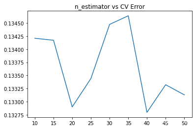
Boosting

Boosting比Bagging理论上更高级点，它也是揽来一把的分类器。但是把他们线性排列。下一个分类器把上一个分类器分类得不好的地方加上更高的权重，这样下一个分类器就能在这个部分学得更加“深刻”。

from sklearn.ensemble import AdaBoostRegressor
params = [10, 15, 20, 25, 30, 35, 40, 45, 50]
test_scores = []
for param in params:
    clf = BaggingRegressor(n_estimators=param, base_estimator=ridge)
    test_score = np.sqrt(-cross_val_score(clf, X_train, y_train, cv=10, scoring='neg_mean_squared_error'))
    test_scores.append(np.mean(test_score))
plt.plot(params, test_scores)
plt.title("n_estimator vs CV Error");

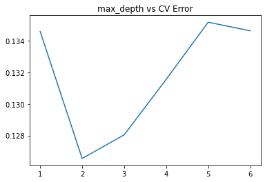
XGBoost

最后，我们来看看巨牛逼的XGBoost，外号：Kaggle神器

这依旧是一款Boosting框架的模型，但是却做了很多的改进。

from xgboost import XGBRegressor

params = [1,2,3,4,5,6]
test_scores = []
for param in params:
    clf = XGBRegressor(max_depth=param)
    test_score = np.sqrt(-cross_val_score(clf, X_train, y_train, cv=10, scoring='neg_mean_squared_error'))
    test_scores.append(np.mean(test_score))

import matplotlib.pyplot as plt
%matplotlib inline
plt.plot(params, test_scores)
plt.title("max_depth vs CV Error");