


kernel参数
对于模型中的kernel参数中默认为"rbf"(高斯核函数),该参数必须是linear(线性) poly rbf三个中的一个
import numpy as np
from matplotlib import pyplot as plt
'''构造数据'''
X1D = np.linspace(-4, 4, 9).reshape(-1, 1)
X2D = np.c_[X1D, X1D ** 2]
y = np.array([0, 0, 1, 1, 1, 1, 1, 0, 0])
from sklearn.datasets import make_moons
X, y = make_moons(n_samples=100, noise=0.15, random_state=42) #指定两个环形测试数据
from sklearn.svm import SVC
from sklearn.pipeline import Pipeline ##使用操作流水线
from sklearn.preprocessing import StandardScaler
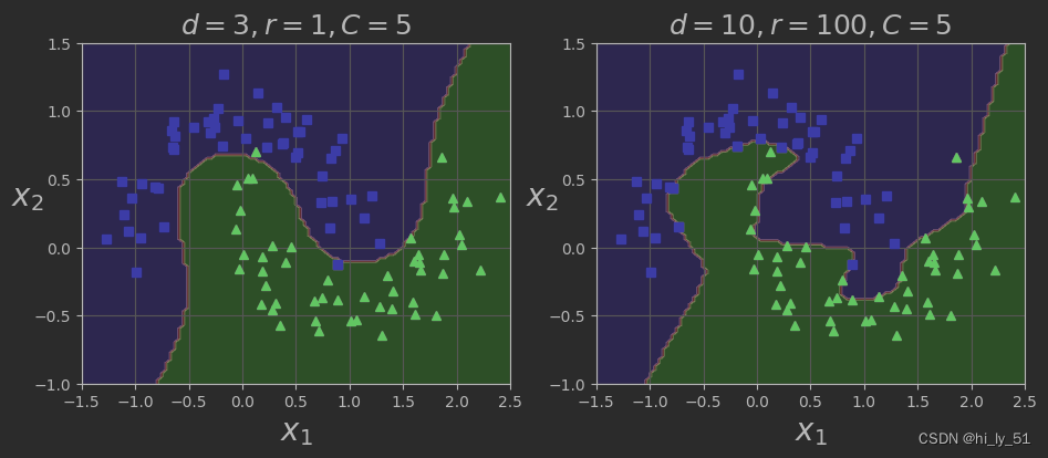
'''通过设置degree值来进行对比实验'''
poly_kernel_svm_clf = Pipeline([
("scaler", StandardScaler()),
("svm_clf", SVC(kernel="poly", degree=3, coef0=1, C=5)) ##coef0表示偏置项
])
poly_kernel_svm_clf.fit(X, y)
poly100_kernel_svm_clf = Pipeline([
("scaler", StandardScaler()),
("svm_clf", SVC(kernel="poly", degree=100, coef0=1, C=5))
])
poly100_kernel_svm_clf.fit(X, y)
###制图展示对比结果
def plot_predictions(clf, axes):
xOs = np.linspace(axes[0], axes[1], 100)
x1s = np.linspace(axes[2], axes[3], 100)
x0, x1 = np.meshgrid(xOs, x1s) ##构建坐标棋盘
X = np.c_[x0.ravel(), x1.ravel()]
y_pred = clf.predict(X).reshape(x0.shape) #一定要对预测结果进行reshape操作
plt.contourf(x0, x1, y_pred, cmap=plt.cm.brg, alpha=0.2)
def plot_dataset(X, y, axes):
plt.plot(X[:, 0][y == 0], X[:, 1][y == 0], "bs")
plt.plot(X[:, 0][y == 1], X[:, 1][y == 1], "g^")
plt.axis(axes)
plt.grid(True, which='both')
plt.xlabel(r"$x_1$", fontsize=20)
plt.ylabel(r"$x_2$", fontsize=20, rotation=0)
plt.figure(figsize=(11, 4))
plt.subplot(121)
plot_predictions(poly_kernel_svm_clf, [-1.5, 2.5, -1, 1.5])
plot_dataset(X, y, [-1.5, 2.5, -1, 1.5])
plt.title(r"$d=3,r=1,C=5$", fontsize=18)
plt.subplot(122)
plot_predictions(poly100_kernel_svm_clf, [-1.5, 2.5, -1, 1.5])
plot_dataset(X, y, [-1.5, 2.5, -1, 1.5])
plt.title(r"$d=10,r=100,C=5$", fontsize=18)
plt.show()相对于对原始数据的操作,使用支持向量机poly变换时对于原始数据并没有改变
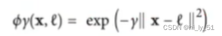
高斯核函数
公式分析
高斯核函数利用相似度来进行变换特征,高斯核函数的基本出发点,对于样本集中的每一个数据,原始都有自己的特征,使用相似度特征来替代样本原始特征。相似度,即当前样本点与其他所有样本点相似度计算得到的特征值。
其运算公式如下:
'''定义高斯核函数'''


def gaussian_rbf(x, landmark, gamma):
    '''

    :param x: 待变换数据
    :param landmark:当前选择位置
    :param gamma:(不同γ值对公式会产生不同的影响)
    :return:
    '''
    return np.exp(-gamma * np.linalg.norm(x - landmark, axis=1) ** 2)


gamma = 0.3

x1s = np.linspace(-4.5, 4.5, 200).reshape(-1, 1)
##分别选择不同的地标将数据进行映射
x2s = gaussian_rbf(x1s, -2, gamma)
x3s = gaussian_rbf(x1s, 1, gamma)

XK = np.c_[gaussian_rbf(X1D, -2, gamma), gaussian_rbf(X1D, 1, gamma)]
yk = np.array([0, 0, 1, 1, 1, 1, 1, 0, 0])

plt.figure(figsize=(11, 4))

###绘制变换前数据分布已经变换过程
plt.subplot(121)
plt.grid(True, which='both')
plt.axhline(y=0, color='k')
plt.scatter(x=[-2, 1], y=[0, 0], s=150, alpha=0.5, c="red")
plt.plot(X1D[:, 0][yk == 0], np.zeros(4), "bs")
plt.plot(X1D[:, 0][yk == 1],np.zeros(5), "g^")
plt.plot(x1s, x2s, "g-")
plt.plot(x1s, x3s, "b:")
plt.gca().get_yaxis().set_ticks([0, 0.25, 0.5, 0.75, 1])
plt.xlabel(r"$x_1$", fontsize=20)
plt.ylabel(r"Similarity", fontsize=14)
plt.annotate(r'$\mathbf{x}$',
             xy=(X1D[3, 0], 0),
             xytext=(-0.5, 0.20),
             ha="center",
             arrowprops=dict(facecolor='black', shrink=0.1),
             fontsize=18, )
plt.text(-2, 0.9, "Sx_2s", ha="center", fontsize=20)
plt.text(1, 0.9, "Sx_3S", ha="center", fontsize=20)
plt.axis([-4.5, 4.5, -0.1, 1.1])

##绘制最终结果与分界线
plt.subplot(122)
plt.grid(True, which='both')
plt.axhline(y=0, color='k')
plt.axvline(x=0, color='k')
plt.plot(XK[:, 0][yk == 0], XK[:, 1][yk == 0], "bs")
plt.plot(XK[:, 0][yk == 1], XK[:, 1][yk == 1], "g^")
plt.xlabel(r"$x_2$", fontsize=20)
plt.ylabel(r"$x_3$", fontsize=20, rotation=0)
plt.annotate(r'$\phi\left (\mathbf{x}\right)$',
             xy=(XK[3, 0], XK[3, 1]),
             xytext=(0.65, 0.50),
             ha="center",
             arrowprops=dict(facecolor='black', shrink=0.1),
             fontsize=18, )
plt.plot([-0.1, 1.1], [0.57, -0.1], "r--", linewidth=3)
plt.axis([-0.1, 1.1, -0.1, 1.1])

plt.subplots_adjust(right=1)

plt.show()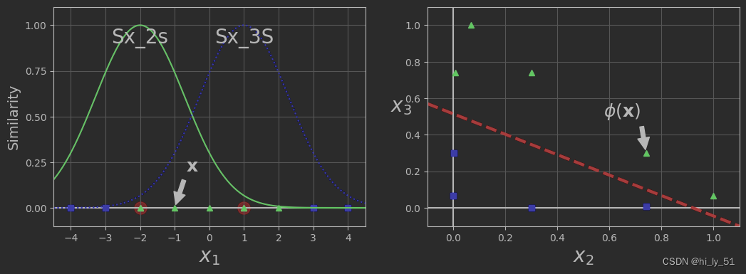
高斯核函数γ值与C值
-
γ值变小,高斯曲线变宽,考虑的更加全面,此实例具有更大的影响范围,并且决策边界更加平滑,模型过拟合风险更低;
-
γ值变大,高斯曲线变窄,因此每个实例的影响范围都较小,决策边界变得更不规则。在个别实例周围摆动,仅针对于个别数据有作用,模型过拟合风险高。
'''探讨γ值与C值对模型结果的影响'''
from sklearn.svm import SVC

gamma1, gamma2 = 0.1, 5
C1, C2 = 0.001, 1000
hyperparams = (gamma1, C1), (gamma1, C2), (gamma2, C1), (gamma2, C2)

svm_clfs = []
for gamma, C in hyperparams:
    rbf_kernel_svm_clf = Pipeline([
        ("scaler", StandardScaler()),
        ("svm_clf", SVC(kernel="rbf", gamma=gamma, C=C))
    ])
    rbf_kernel_svm_clf.fit(X, y)
    svm_clfs.append(rbf_kernel_svm_clf)
plt.figure(figsize=(11, 7))

for i, svm_clf in enumerate(svm_clfs):
    plt.subplot(221 + i)
    plot_predictions(svm_clf, [-1.5, 2.5, -1, 1.5])
    plot_dataset(X, y, [-1.5, 2.5, -1, 1.5])
    gamma, C = hyperparams[i]
    plt.title(r'$\gamma={},C={}$'.format(gamma, C), fontsize=16)
plt.show()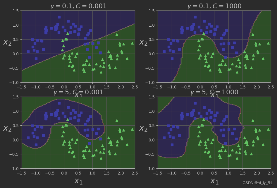


 2011
2011

 被折叠的 条评论
为什么被折叠?
被折叠的 条评论
为什么被折叠?
 到【灌水乐园】发言


