


参考来源:
动手深度学习(第二版)
一、Softmax回归基本步骤和原理
1、引言
在前文中,我们已经学习过回归的线性问题该如何预测,但在现实中很多问题并不是需要去猜测数值大小,而是考虑是哪种。如某个电子邮件是否属于垃圾邮件文件夹,某个用户可能注册或不注册订阅服务等等。为了表示分类数据,我们需要用到独热编码(one-hot encoding)。
独热编码是一个向量,它的分量和类别一样多。 类别对应的分量设置为1,其他所有分量设置为0。加假如有三个类别,那么(1,0,0)表示第一个类别,(0,1,0)为第二个,(0,0,1)为第三个则为(0,0,1)
2、Softmax回归的优缺点
优点:
- Softmax回归比较容易实现和理解,模型结构简单。
- 适用于多分类任务,能够对数据进行良好的分类。
- 可使用梯度下降等优化算法对模型进行训练,提高预测准确性。
缺点:
- Softmax回归只适用于线性可分的数据,在处理复杂非线性问题时会出现一定局限性。
- 如果特征空间较大,参数数量会变得非常庞大,需要更多的数据进行训练以防止过拟合。
- 当数据类别不平衡时,通过权重调整可以改善这个问题,但也会加大模型复杂度。同时,数据类别很少或不存在某一个类别时,则无法进行有效的预测。
3、基本步骤
Softmax回归的步骤如下:
-
首先将输入特征向量经过线性变换,得出每个类别的得分。即对于 ii 类别的得分为: z_i = w_i^Tx+b_izi=wiTx+bi
-
然后将得分用exponential函数进行指数化,即 e^{z_i}ezi
-
对所有得分求和:\sum_j e^{z_j}∑jezj
-
按照softmax公式计算每个类别的概率:
P(i)=\frac{e^{z_i}}{\sum_j e^{z_j}}P(i)=∑jezjezi
通过这些步骤,我们就可以得到每个类别的预测概率。
4、网络架构
与线性回归不同的是,线性回归往往只需要预测出一个结果,所以为单输出模型。在Softmax回归中,为了估计所有可能类别的条件概率,我们需要一个有多个输出的模型,每个类别对应一个输出。这时,我们就需要有结果数量个放射函数来确定如何才能映射到对应的类别上面。下图为三个类别,每个类别具有四个样本时的情况:

神经网络图如下所示:
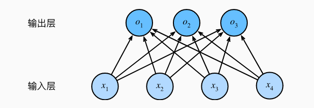
在计算中通过向量形式表达为o=Wx+b。
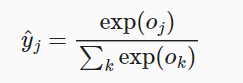
5、Sofemax运算
为了使输出得到的o可以作为概率判别的依据,我需要将其规范化。将输出视为概率,我们必须保证在任何数据上的输出都是非负的且总和为1。 此外,我们需要一个训练的目标函数,来激励模型精准地估计概率。为此,我们需要对数据作如下变换,使得其得到结果为概率分布。
6、损失函数
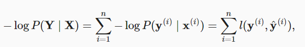
与线性回归一样,仍采用极大似然估计法推导。softmax函数给出了一个向量y^, 我们可以将其视为“对给定任意输入x的每个类的条件概率”。 例如,y^1=猫P(y=猫∣x)。 假设整个数据集{X,Y}具有n个样本, 其中索引i的样本由特征向量x(i)和独热标签向量y(i)组成。 我们可以将估计值与实际值进行比较:

根据最大似然估计,我们最大化P(Y∣X),相当于最小化负对数似然:
其中,对于任何标签y和模型预测y^,损失函数为:
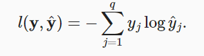
这种损失函数被称为交叉熵损失(cross-entropy loss),之后我们将规范化后的y带入式子中,得到:


二、代码实现
复杂版:
import torch
from IPython import display
from d2l import torch as d2l
batch_size = 256
train_iter, test_iter = d2l.load_data_fashion_mnist(batch_size)
num_inputs = 784
num_outputs = 10

W = torch.normal(0, 0.01, size=(num_inputs, num_outputs), requires_grad=True)
#输入需要是向量
b = torch.zeros(num_outputs, requires_grad=True)
def softmax(X):
    X_exp = torch.exp(X)
    partition = X_exp.sum(1, keepdim=True)
    return X_exp / partition  # 这里应用了广播机制
def net(X):
    return softmax(torch.matmul(X.reshape((-1, W.shape[0])), W) + b)
def cross_entropy(y_hat, y):
    return - torch.log(y_hat[range(len(y_hat)), y])

cross_entropy(y_hat, y)
def accuracy(y_hat, y):  #@save
    """计算预测正确的数量"""
    if len(y_hat.shape) > 1 and y_hat.shape[1] > 1:
        y_hat = y_hat.argmax(axis=1)
    cmp = y_hat.type(y.dtype) == y
    return float(cmp.type(y.dtype).sum())
def evaluate_accuracy(net, data_iter):  #@save
    """计算在指定数据集上模型的精度"""
    if isinstance(net, torch.nn.Module):
        net.eval()  # 将模型设置为评估模式
    metric = Accumulator(2)  # 正确预测数、预测总数
    with torch.no_grad():
        for X, y in data_iter:
            metric.add(accuracy(net(X), y), y.numel())
    return metric[0] / metric[1]
class Accumulator:  #@save
    """在n个变量上累加"""
    def __init__(self, n):
        self.data = [0.0] * n

    def add(self, *args):
        self.data = [a + float(b) for a, b in zip(self.data, args)]

    def reset(self):
        self.data = [0.0] * len(self.data)

    def __getitem__(self, idx):
        return self.data[idx]
accuracy(y_hat, y) / len(y)
evaluate_accuracy(net, test_iter)
def train_epoch_ch3(net, train_iter, loss, updater):  #@save
    """训练模型一个迭代周期(定义见第3章)"""
    # 将模型设置为训练模式
    if isinstance(net, torch.nn.Module):
        net.train()
    # 训练损失总和、训练准确度总和、样本数
    metric = Accumulator(3)
    for X, y in train_iter:
        # 计算梯度并更新参数
        y_hat = net(X)
        l = loss(y_hat, y)
        if isinstance(updater, torch.optim.Optimizer):
            # 使用PyTorch内置的优化器和损失函数
            updater.zero_grad()
            l.mean().backward()
            updater.step()
        else:
            # 使用定制的优化器和损失函数
            l.sum().backward()
            updater(X.shape[0])
        metric.add(float(l.sum()), accuracy(y_hat, y), y.numel())
    # 返回训练损失和训练精度
    return metric[0] / metric[2], metric[1] / metric[2]
class Animator:  #@save
    """在动画中绘制数据"""
    def __init__(self, xlabel=None, ylabel=None, legend=None, xlim=None,
                 ylim=None, xscale='linear', yscale='linear',
                 fmts=('-', 'm--', 'g-.', 'r:'), nrows=1, ncols=1,
                 figsize=(3.5, 2.5)):
        # 增量地绘制多条线
        if legend is None:
            legend = []
        d2l.use_svg_display()
        self.fig, self.axes = d2l.plt.subplots(nrows, ncols, figsize=figsize)
        if nrows * ncols == 1:
            self.axes = [self.axes, ]
        # 使用lambda函数捕获参数
        self.config_axes = lambda: d2l.set_axes(
            self.axes[0], xlabel, ylabel, xlim, ylim, xscale, yscale, legend)
        self.X, self.Y, self.fmts = None, None, fmts

    def add(self, x, y):
        # 向图表中添加多个数据点
        if not hasattr(y, "__len__"):
            y = [y]
        n = len(y)
        if not hasattr(x, "__len__"):
            x = [x] * n
        if not self.X:
            self.X = [[] for _ in range(n)]
        if not self.Y:
            self.Y = [[] for _ in range(n)]
        for i, (a, b) in enumerate(zip(x, y)):
            if a is not None and b is not None:
                self.X[i].append(a)
                self.Y[i].append(b)
        self.axes[0].cla()
        for x, y, fmt in zip(self.X, self.Y, self.fmts):
            self.axes[0].plot(x, y, fmt)
        self.config_axes()
        display.display(self.fig)
        display.clear_output(wait=True)
def train_ch3(net, train_iter, test_iter, loss, num_epochs, updater):  #@save
    """训练模型(定义见第3章)"""
    animator = Animator(xlabel='epoch', xlim=[1, num_epochs], ylim=[0.3, 0.9],
                        legend=['train loss', 'train acc', 'test acc'])
    for epoch in range(num_epochs):
        train_metrics = train_epoch_ch3(net, train_iter, loss, updater)
        test_acc = evaluate_accuracy(net, test_iter)
        animator.add(epoch + 1, train_metrics + (test_acc,))
    train_loss, train_acc = train_metrics
    assert train_loss < 0.5, train_loss
    assert train_acc <= 1 and train_acc > 0.7, train_acc
    assert test_acc <= 1 and test_acc > 0.7, test_acc
lr = 0.1

def updater(batch_size):
    return d2l.sgd([W, b], lr, batch_size)
num_epochs = 20
train_ch3(net, train_iter, test_iter, cross_entropy, num_epochs, updater)
def predict_ch3(net, test_iter, n=6):  #@save
    """预测标签(定义见第3章)"""
    for X, y in test_iter:
        break
    trues = d2l.get_fashion_mnist_labels(y)
    preds = d2l.get_fashion_mnist_labels(net(X).argmax(axis=1))
    titles = [true +'\n' + pred for true, pred in zip(trues, preds)]
    d2l.show_images(
        X[0:n].reshape((n, 28, 28)), 1, n, titles=titles[0:n])

predict_ch3(net, test_iter)
简洁版:
import torch
from torch import nn
from d2l import torch as d2l
batch_size = 256
train_iter, test_iter = d2l.load_data_fashion_mnist(batch_size)

# PyTorch不会隐式地调整输入的形状。因此,
# 我们在线性层前定义了展平层(flatten),来调整网络输入的形状
net = nn.Sequential(nn.Flatten(), nn.Linear(784, 10))

# PyTorch不会隐式地调整输入的形状。因此,
# 我们在线性层前定义了展平层(flatten),来调整网络输入的形状
net = nn.Sequential(nn.Flatten(), nn.Linear(784, 10))

def init_weights(m):
    if type(m) == nn.Linear:
        #把wight初始化为均值为零方差为0.01的均差函数
        nn.init.normal_(m.weight, std=0.01)

net.apply(init_weights);

loss = nn.CrossEntropyLoss(reduction='none')

trainer = torch.optim.SGD(net.parameters(), lr=0.1)

num_epochs = 10
d2l.train_ch3(net, train_iter, test_iter, loss, num_epochs, trainer)


 5636
5636


 被折叠的 条评论
为什么被折叠?
被折叠的 条评论
为什么被折叠?
 到【灌水乐园】发言


