


文章目录
在做 多个变量(n > 3) 的链式中介时,初期为了探索所有可能的结果,我们就需要设计 n ! n! n!个模型。
例如:如果我有四个变量,就要设计
4
∗
3
∗
2
∗
1
=
24
4*3*2*1=24
4∗3∗2∗1=24 种模型,手动设计的话非常浪费时间。在此,我以四个变量为例,设计了一个函数,填入四个变量后,模型就可以一次性跑出所有的结果。
声明:本文仅为学习笔记,可供参考。欢迎各位大佬批评指正。
一、位置固定的链式中介
首先,我将以确定了自变量、因变量以及两个中介变量先后顺序的链式中介模型为例,说明在R中如何利用 bruceR 和 ggplot2 包设计链式中介模型并作图。
1.1 安装特定包
#install.packages("bruceR")
#install.packages("ggplot2")
#install.packages("dplyr")
library("bruceR")
library("ggplot2")
library("dplyr")
1.2 提取数据
这里以mediation::student中的demo data为例。
data = mediation::student %>%
  dplyr::select (pared,income,late, score) #使用dplyr包中的select选择这四个变量
names(data)[1:2] = c("parent_edu", "family_inc") #将前两个变量改名
bruceR::Describe(data) #使用bruceR包中的Describe对这几个变量进行描述性统计
1.3 链式中介
#将model的结果输入进入"result"这个变量
result<-bruceR::PROCESS(data, y="score", x="parent_edu",#y因变量和x自变量
        meds=c("family_inc", "late"), #两个中介变量(有先后顺序)
        med.type="serial",            #中介类型,serial为链式中介
        ci="boot", nsim=100, seed=1)  #ci选择Bootstrap的类型;
                                      #nsim是Bootstrap的数量,
                                      #这里为了节省时间设置为100,正常情况下nsim > 1000
                                      #seed=1设定随机种子让模型的结果有可重复性
1.4结果解读
1.4.1 Model Summary

1.4.2 Mediation Effect Estimate

该图中的每个字母分别代表以下路径的回归系数。


在该模型中,只有X->M2->Y这条路径的95%CI包含0,不显著。
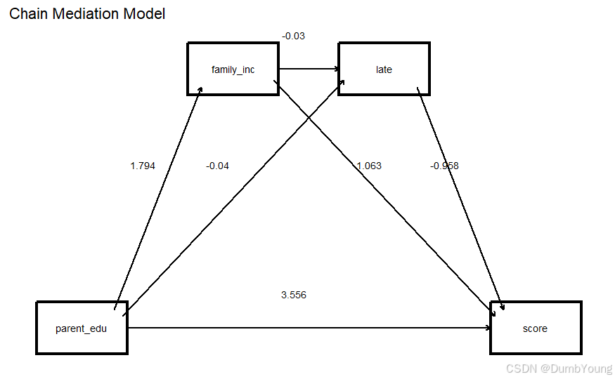
1.5 作图
图中包含路径和路径系数。
只有path_coefficients部分需要根据自己的变量名称和路径方向进行调整。
只是个草图,在初期探索是适用。若想要做更精美的图可添加更多参数(或使用PPT等绘图软件)
# 计算箭头的起点和终点,基于矩形框边缘调整
# 参数:
#   x1, y1: 起点的坐标 (矩形中心)
#   x2, y2: 终点的坐标 (矩形中心)
#   box_width, box_height: 矩形框的宽度和高度,用于调整边界
adjust_arrow <- function(x1, y1, x2, y2, box_width = 0.6, box_height = 0.2) {
  # 计算箭头方向的角度
  angle <- atan2(y2 - y1, x2 - x1)

  # 根据矩形的宽度和高度,调整箭头的起点和终点,使其从边框开始
  x_start <- x1 + (box_width / 2) * cos(angle)
  y_start <- y1 + (box_height / 2) * sin(angle)
  x_end <- x2 - (box_width / 2) * cos(angle)
  y_end <- y2 - (box_height / 2) * sin(angle)

  # 返回计算后的起点和终点坐标
  return(list(x_start = x_start, y_start = y_start, x_end = x_end, y_end = y_end))
}

# 路径系数数据框,包含从某个变量到另一个变量的路径及其系数
# 四个变量共有六条路径
path_coefficients <- data.frame(
  from = factor(c("parent_edu", "parent_edu", "family_inc", "parent_edu", "family_inc", "late")),#六条路径的起始点(不可打乱顺序)
  to = factor(c("family_inc", "late", "late", "score", "score", "score")),#六条路径的结束点(不可打乱顺序)
  estimate = c(
    result$model.m$model.m.1$coefficients["parent_edu"],  # parent_edu -> family_inc
    result$model.m$model.m.2$coefficients["parent_edu"],  # parent_edu -> late
    result$model.m$model.m.2$coefficients["family_inc"],   # family_inc -> late
    result$model.y$coefficients["parent_edu"],            # parent_edu -> score
    result$model.y$coefficients["family_inc"],             # family_inc -> score
    result$model.y$coefficients["late"]                 # late -> score
  )#从result中提取这六条路径的回归系数(不可打乱顺序)
)

# 变量的坐标数据框,定义每个变量在图中的位置
variables <- data.frame(
  name = c("parent_edu", "family_inc", "late", "score"),
  x = c(1, 2, 3, 4),  # x坐标
  y = c(2, 3, 3, 2)   # y坐标
)

# 通过循环遍历路径系数,调整箭头的起点和终点位置
adjusted_arrows <- do.call(rbind, lapply(1:nrow(path_coefficients), function(i) {
  # 获取起点和终点在变量中的索引
  from_index <- match(path_coefficients$from[i], variables$name)
  to_index <- match(path_coefficients$to[i], variables$name)

  # 计算调整后的箭头坐标
  coords <- adjust_arrow(variables$x[from_index], variables$y[from_index],
                         variables$x[to_index], variables$y[to_index])

  # 创建新的数据框,包含调整后的起点和终点坐标
  data.frame(
    x = coords$x_start, y = coords$y_start,
    xend = coords$x_end, yend = coords$y_end,
    estimate = path_coefficients$estimate[i]  # 路径系数
  )
}))

# 绘制路径模型图
ggplot() +
  # 绘制每个变量的矩形框
  geom_rect(data = variables,
            aes(xmin = x - 0.3, xmax = x + 0.3, ymin = y - 0.1, ymax = y + 0.1),  # 矩形的大小和位置
            fill = "white", color = "black", size = 1.2) +  # 矩形的样式

  # 在每个矩形框中添加变量名称
  geom_text(data = variables,
            aes(x = x, y = y, label = name),  # 变量名称的位置和内容
            size = 3) +  # 文本大小

  # 绘制路径箭头,固定线条宽度为0.8
  geom_segment(data = adjusted_arrows,
               aes(x = x, y = y, xend = xend, yend = yend),  # 箭头的起点和终点
               linewidth = 0.8,  # 固定箭头的线条宽度为0.8
               arrow = arrow(length = unit(0.15, "cm")),  # 箭头的样式和大小
               color = "black") +  # 线条颜色为黑色

  # 添加路径系数标注,避免被遮挡
  geom_text(data = adjusted_arrows,
            aes(x = (x + xend) / 2 - 0.1,  # 箭头中点的x坐标
                 y = (y + yend) / 2 + 0.1,  # 箭头中点的y坐标,稍微偏移避免重叠
                 label = round(estimate, 3)),  # 标注路径系数,保留两位小数
            vjust = -0.5, size = 3, color = "black") +  # 文本样式

  # 设置主题样式,移除坐标轴和网格线
  theme_minimal() +
  labs(title = "Chain Mediation Model") +  # 添加标题
  theme(axis.text = element_blank(), axis.ticks = element_blank(),  # 隐藏坐标轴文本和刻度
        axis.title = element_blank(), panel.grid = element_blank())  # 隐藏坐标轴标题和网格线
二、4变量24种结果1次解决函数
在一部分,我们已经解决了如果确定自变量和因变量,以及两个中介变量先后顺序的模型应该怎么计算和制作。在本部分,就回到文章主题,如何通过函数一次性计算24种不同结果。
2.1 安装特定包
#install.packages("bruceR")
#install.packages("ggplot2")
#install.packages("dplyr")
library("bruceR")
library("ggplot2")
library("dplyr")
2.2 提取数据
仍然以mediation::student中的demo data为例。
data = mediation::student %>%
  dplyr::select (pared,income,late, score) #使用dplyr包中的select选择这四个变量
names(data)[1:2] = c("parent_edu", "family_inc") #将前两个变量改名
bruceR::Describe(data) #使用bruceR包中的Describe对这几个变量进行描述性统计
2.3 1次性计算24个中介模型的结果并作图
只需要在最后定义variables的name
# 加载所需的R包,这些包为我们提供了函数来执行中介分析、生成图表和排列组合
library(bruceR) # 用于中介分析 (PROCESS 函数)
library(ggplot2) # 用于生成图表 (绘制路径模型图)
#install.packages("gtools")
library(gtools) # 用于生成排列组合 (permutations 函数)
# 定义函数,重新计算每个组合的中介分析参数并绘制路径模型
draw_mediation_model <- function(x, y, med1, med2, data) {
# 使用 bruceR 包的 PROCESS 函数进行中介分析,分析 x 如何通过 med1 和 med2 影响 y
result <- bruceR::PROCESS(data,
y = y, # 因变量,最终受到影响的变量
x = x, # 自变量,最初引起影响的变量
meds = c(med1, med2), # 两个中介变量 med1 和 med2
med.type = "serial", # 串联中介,即 med1 影响 med2,med2 影响 y
ci = "boot", # 使用 bootstrap 方法计算置信区间
nsim = 100, # 设置 bootstrap 重采样次数为 100
seed = 1) # 设置随机种子,确保结果可重复
# 构建一个数据框,存储从自变量到因变量(包括中介变量)的路径系数
# 这里定义了6条路径,比如 x -> med1, med1 -> med2 等
path_coefficients <- data.frame(
from = factor(c(x, x, med1, x, med1, med2)), # 路径起点
to = factor(c(med1, med2, med2, y, y, y)), # 路径终点
estimate = c(
result$model.m$model.m.1$coefficients[x], # x -> med1 的系数
result$model.m$model.m.2$coefficients[x], # x -> med2 的系数
result$model.m$model.m.2$coefficients[med1], # med1 -> med2 的系数
result$model.y$coefficients[x], # x -> y 的系数
result$model.y$coefficients[med1], # med1 -> y 的系数
result$model.y$coefficients[med2] # med2 -> y 的系数
)
)
# 定义每个变量在图中的坐标位置 (x 和 y 轴坐标)
variables <- data.frame(
name = c(x, med1, med2, y), # 变量名:自变量、中介1、中介2、因变量
x = c(1, 2, 3, 4), # 每个变量在 x 轴上的位置
y = c(2, 3, 3, 2) # 每个变量在 y 轴上的位置
)
# 调整箭头位置的函数,确保箭头从框的边缘开始
# 箭头从起点框的边缘出发,到达终点框的边缘,而不是直接从中心到中心
adjust_arrow <- function(x1, y1, x2, y2, box_width = 0.6, box_height = 0.2) {
angle <- atan2(y2 - y1, x2 - x1) # 计算两个点之间的角度
x_start <- x1 + (box_width / 2) * cos(angle) # 调整起点的 x 坐标
y_start <- y1 + (box_height / 2) * sin(angle) # 调整起点的 y 坐标
x_end <- x2 - (box_width / 2) * cos(angle) # 调整终点的 x 坐标
y_end <- y2 - (box_height / 2) * sin(angle) # 调整终点的 y 坐标
return(list(x_start = x_start, y_start = y_start, x_end = x_end, y_end = y_end))
}
# 计算调整后的箭头坐标
# 遍历所有路径,调整箭头的起点和终点
adjusted_arrows <- do.call(rbind, lapply(1:nrow(path_coefficients), function(i) {
from_index <- match(path_coefficients$from[i], variables$name) # 找到路径起点的索引
to_index <- match(path_coefficients$to[i], variables$name) # 找到路径终点的索引
coords <- adjust_arrow(variables$x[from_index], variables$y[from_index],
variables$x[to_index], variables$y[to_index]) # 计算箭头的起止位置
data.frame(
x = coords$x_start, y = coords$y_start, # 箭头起点坐标
xend = coords$x_end, yend = coords$y_end, # 箭头终点坐标
estimate = path_coefficients$estimate[i] # 该路径的估计系数
)
}))
# 使用 ggplot2 绘制路径模型图
ggplot() +
# 绘制每个变量的矩形框,表示变量的位置
geom_rect(data = variables,
aes(xmin = x - 0.3, xmax = x + 0.3, ymin = y - 0.1, ymax = y + 0.1),
fill = "white", color = "black", size = 1.2) +
# 在每个矩形框中间标注变量的名称
geom_text(data = variables,
aes(x = x, y = y, label = name),
size = 3) +
# 绘制路径的箭头,表示变量之间的因果关系
geom_segment(data = adjusted_arrows,
aes(x = x, y = y, xend = xend, yend = yend),
size = 0.8,
arrow = arrow(length = unit(0.15, "cm")),
color = "black") +
# 在路径旁边标注路径的估计系数
geom_text(data = adjusted_arrows,
aes(x = (x + xend) / 2 - 0.1,
y = (y + yend) / 2 + 0.1,
label = round(estimate, 3)),
vjust = -0.5, size = 3, color = "black") +
# 设置图表的基本样式
theme_minimal() +
# 设置图表的标题,表示模型链
labs(title = paste("Chain Mediation Model:", x, "->", med1, "->", med2, "->", y)) +
# 移除坐标轴和网格线
theme(axis.text = element_blank(), axis.ticks = element_blank(),
axis.title = element_blank(), panel.grid = element_blank())
}
# 定义主函数,接受四个变量,生成所有组合并绘制路径模型
generate_all_models <- function(variables, data) {
# 获取变量的所有排列组合,确保每个组合有不同的自变量、因变量和两个中介变量
perms <- permutations(length(variables), length(variables), variables)
# 遍历每个排列组合,调用绘制函数生成路径模型
for (i in 1:nrow(perms)) {
# 取出排列组合中的自变量、因变量和两个中介变量
x <- perms[i, 1] # 自变量
y <- perms[i, 4] # 因变量
med1 <- perms[i, 2] # 中介变量1
med2 <- perms[i, 3] # 中介变量2
# 调用绘制函数,传入数据和变量进行绘制
print(draw_mediation_model(x, y, med1, med2, data))
}
}
# 定义要使用的变量名称
variables <- c("parent_edu", "family_inc", "late", "score")
# 调用主函数,生成所有组合并绘制路径模型
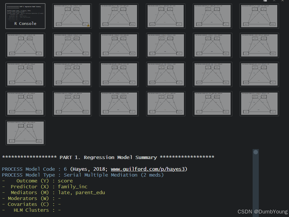
generate_all_models(variables, data)
结果:


 703
703

 被折叠的 条评论
为什么被折叠?
被折叠的 条评论
为什么被折叠?
 到【灌水乐园】发言


