k臂赌博机问题学习笔记以及代码运行

 

python代码实现：

 #######################################################################
# Copyright (C)                                                       #
# 2016-2018 Shangtong Zhang(zhangshangtong.cpp@gmail.com)             #
# 2016 Tian Jun(tianjun.cpp@gmail.com)                                #
# 2016 Artem Oboturov(oboturov@gmail.com)                             #
# 2016 Kenta Shimada(hyperkentakun@gmail.com)                         #
# Permission given to modify the code as long as you keep this        #
# declaration at the top                                              #
#######################################################################

import matplotlib
import matplotlib.pyplot as plt
import numpy as np
from tqdm import trange

matplotlib.use('Agg')


class Bandit:
    # @k_arm: # of arms
    # @epsilon: probability for exploration in epsilon-greedy algorithm
    # @initial: initial estimation for each action
    # @step_size: constant step size for updating estimations
    # @sample_averages: if True, use sample averages to update estimations instead of constant step size
    # @UCB_param: if not None, use UCB algorithm to select action
    # @gradient: if True, use gradient based bandit algorithm
    # @gradient_baseline: if True, use average reward as baseline for gradient based bandit algorithm
    def __init__(self, k_arm=10, epsilon=0., initial=0., step_size=0.1, sample_averages=False, UCB_param=None,
                 gradient=False, gradient_baseline=False, true_reward=0.):
        self.k = k_arm
        self.step_size = step_size
        self.sample_averages = sample_averages
        self.indices = np.arange(self.k)
        self.time = 0
        self.UCB_param = UCB_param
        self.gradient = gradient
        self.gradient_baseline = gradient_baseline
        self.average_reward = 0
        self.true_reward = true_reward
        self.epsilon = epsilon
        self.initial = initial

    def reset(self):
        # real reward for each action
        self.q_true = np.random.randn(self.k) + self.true_reward

        # estimation for each action
        self.q_estimation = np.zeros(self.k) + self.initial

        # # of chosen times for each action
        self.action_count = np.zeros(self.k)

        self.best_action = np.argmax(self.q_true)

        self.time = 0

    # get an action for this bandit
    def act(self):
        if np.random.rand() < self.epsilon:
            return np.random.choice(self.indices)

        if self.UCB_param is not None:
            UCB_estimation = self.q_estimation + \
                self.UCB_param * np.sqrt(np.log(self.time + 1) / (self.action_count + 1e-5))
            q_best = np.max(UCB_estimation)
            return np.random.choice(np.where(UCB_estimation == q_best)[0])

        if self.gradient:
            exp_est = np.exp(self.q_estimation)
            self.action_prob = exp_est / np.sum(exp_est)
            return np.random.choice(self.indices, p=self.action_prob)

        q_best = np.max(self.q_estimation)
        return np.random.choice(np.where(self.q_estimation == q_best)[0])

    # take an action, update estimation for this action
    def step(self, action):
        # generate the reward under N(real reward, 1)
        reward = np.random.randn() + self.q_true[action]
        self.time += 1
        self.action_count[action] += 1
        self.average_reward += (reward - self.average_reward) / self.time

        if self.sample_averages:
            # update estimation using sample averages
            self.q_estimation[action] += (reward - self.q_estimation[action]) / self.action_count[action]
        elif self.gradient:
            one_hot = np.zeros(self.k)
            one_hot[action] = 1
            if self.gradient_baseline:
                baseline = self.average_reward
            else:
                baseline = 0
            self.q_estimation += self.step_size * (reward - baseline) * (one_hot - self.action_prob)
        else:
            # update estimation with constant step size
            self.q_estimation[action] += self.step_size * (reward - self.q_estimation[action])
        return reward


def simulate(runs, time, bandits):
    rewards = np.zeros((len(bandits), runs, time))
    best_action_counts = np.zeros(rewards.shape)
    for i, bandit in enumerate(bandits):
        for r in trange(runs):
            bandit.reset()
            for t in range(time):
                action = bandit.act()
                reward = bandit.step(action)
                rewards[i, r, t] = reward
                if action == bandit.best_action:
                    best_action_counts[i, r, t] = 1
    mean_best_action_counts = best_action_counts.mean(axis=1)
    mean_rewards = rewards.mean(axis=1)
    return mean_best_action_counts, mean_rewards


def figure_2_1():
    plt.violinplot(dataset=np.random.randn(200, 10) + np.random.randn(10))
    plt.xlabel("Action")
    plt.ylabel("Reward distribution")
    plt.savefig('../images/figure_2_1.png')

    plt.close()


def figure_2_2(runs=2000, time=1000):
    epsilons = [0, 0.1, 0.01]
    bandits = [Bandit(epsilon=eps, sample_averages=True) for eps in epsilons]
    best_action_counts, rewards = simulate(runs, time, bandits)

    plt.figure(figsize=(10, 20))

    plt.subplot(2, 1, 1)
    for eps, rewards in zip(epsilons, rewards):
        plt.plot(rewards, label='$\epsilon = %.02f$' % (eps))
    plt.xlabel('steps')
    plt.ylabel('average reward')
    plt.legend()

    plt.subplot(2, 1, 2)
    for eps, counts in zip(epsilons, best_action_counts):
        plt.plot(counts, label='$\epsilon = %.02f$' % (eps))
    plt.xlabel('steps')
    plt.ylabel('% optimal action')
    plt.legend()

    plt.savefig('../images/figure_2_2.png')

    plt.close()


def figure_2_3(runs=2000, time=1000):
    bandits = []
    bandits.append(Bandit(epsilon=0, initial=5, step_size=0.1))
    bandits.append(Bandit(epsilon=0.1, initial=0, step_size=0.1))
    best_action_counts, _ = simulate(runs, time, bandits)

    plt.plot(best_action_counts[0], label='$\epsilon = 0, q = 5$')
    plt.plot(best_action_counts[1], label='$\epsilon = 0.1, q = 0$')
    plt.xlabel('Steps')
    plt.ylabel('% optimal action')
    plt.legend()

    plt.savefig('../images/figure_2_3.png')

    plt.close()


def figure_2_4(runs=2000, time=1000):
    bandits = []
    bandits.append(Bandit(epsilon=0, UCB_param=2, sample_averages=True))
    bandits.append(Bandit(epsilon=0.1, sample_averages=True))
    _, average_rewards = simulate(runs, time, bandits)

    plt.plot(average_rewards[0], label='UCB $c = 2$')
    plt.plot(average_rewards[1], label='epsilon greedy $\epsilon = 0.1$')
    plt.xlabel('Steps')
    plt.ylabel('Average reward')
    plt.legend()

    plt.savefig('../images/figure_2_4.png')

    plt.close()


def figure_2_5(runs=2000, time=1000):
    bandits = []
    bandits.append(Bandit(gradient=True, step_size=0.1, gradient_baseline=True, true_reward=4))
    bandits.append(Bandit(gradient=True, step_size=0.1, gradient_baseline=False, true_reward=4))
    bandits.append(Bandit(gradient=True, step_size=0.4, gradient_baseline=True, true_reward=4))
    bandits.append(Bandit(gradient=True, step_size=0.4, gradient_baseline=False, true_reward=4))
    best_action_counts, _ = simulate(runs, time, bandits)
    labels = [r'$\alpha = 0.1$, with baseline',
              r'$\alpha = 0.1$, without baseline',
              r'$\alpha = 0.4$, with baseline',
              r'$\alpha = 0.4$, without baseline']

    for i in range(len(bandits)):
        plt.plot(best_action_counts[i], label=labels[i])
    plt.xlabel('Steps')
    plt.ylabel('% Optimal action')
    plt.legend()

    plt.savefig('../images/figure_2_5.png')

    plt.close()


def figure_2_6(runs=2000, time=1000):
    labels = ['epsilon-greedy', 'gradient bandit',
              'UCB', 'optimistic initialization']
    generators = [lambda epsilon: Bandit(epsilon=epsilon, sample_averages=True),
                  lambda alpha: Bandit(gradient=True, step_size=alpha, gradient_baseline=True),
                  lambda coef: Bandit(epsilon=0, UCB_param=coef, sample_averages=True),
                  lambda initial: Bandit(epsilon=0, initial=initial, step_size=0.1)]
    parameters = [np.arange(-7, -1, dtype=np.float64),
                  np.arange(-5, 2, dtype=np.float64),
                  np.arange(-4, 3, dtype=np.float64),
                  np.arange(-2, 3, dtype=np.float64)]

    bandits = []
    for generator, parameter in zip(generators, parameters):
        for param in parameter:
            bandits.append(generator(pow(2, param)))

    _, average_rewards = simulate(runs, time, bandits)
    rewards = np.mean(average_rewards, axis=1)

    i = 0
    for label, parameter in zip(labels, parameters):
        l = len(parameter)
        plt.plot(parameter, rewards[i:i+l], label=label)
        i += l
    plt.xlabel('Parameter($2^x$)')
    plt.ylabel('Average reward')
    plt.legend()

    plt.savefig('../images/figure_2_6.png')

    plt.close()


if __name__ == '__main__':
    figure_2_1()
    figure_2_2()
    figure_2_3()
    figure_2_4()
    figure_2_5()
    figure_2_6()

 输出的结果为：

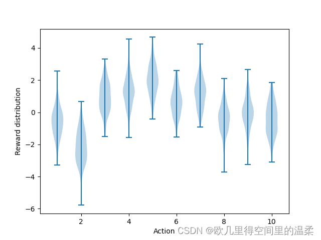
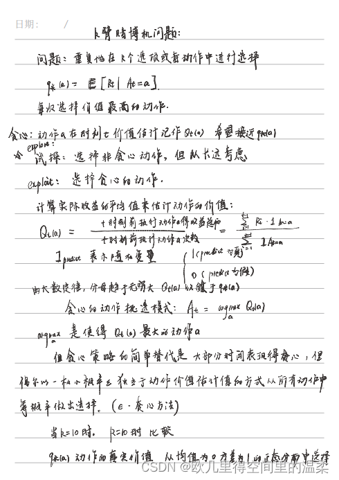
 该图片展示了一个十臂赌博机的测试平台。这十个动作的真实值q*a分别由一个零均值单位方差的正态分布中产生。实际收益由均值为q*(a)的单位方差正态分布当中产生。所有采样方法都用采样平均策略来形成对动作价值的估计。

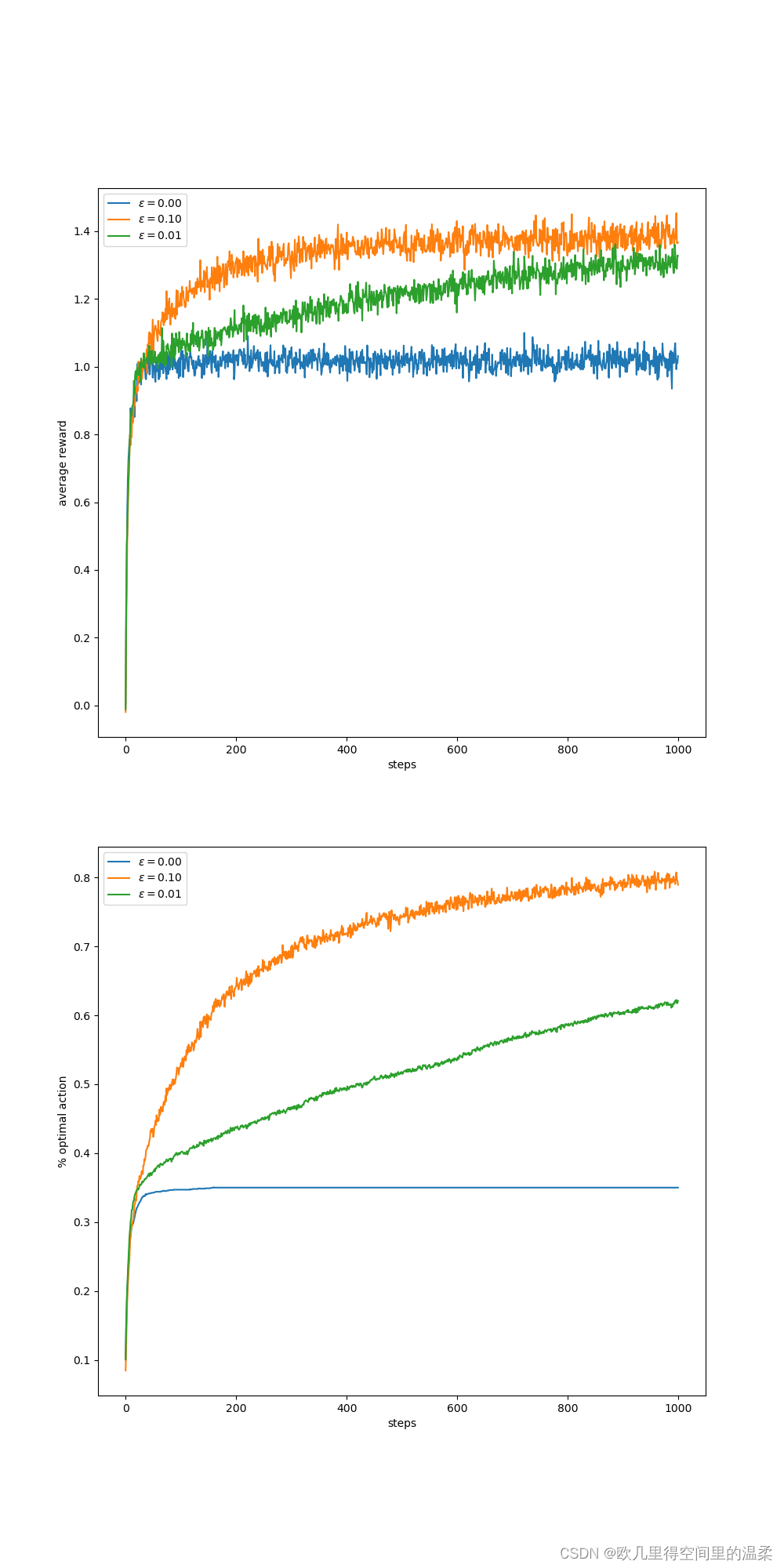
该图比较了贪心算法和贪心算法的对比，贪心算法在最初增长的略微快一些，但是随后稳定在一个较低的水平。从长远来看表现更糟，因为它经常陷入执行次优的怪圈。而贪心算法相对与贪心算法的优点在于依赖于任务。为了找到最优的动作需要更多次的试探。

非平稳性是强化学习中遇到的最常见的状况，即使每一个单独的子任务都会随着学习的平稳推进而有所变化。这使得智能体的兼容也会不断变化。强化学习需要在开发和试探当中取得平衡。

图2.3显示了乐观的初始动作-价值估计在10臂赌博机测试平台上的运行成果。两种方法都采用了恒定步长的参数a=0.1

乐观初始值在平稳的问题当中非常有效，但它远非鼓励试探的普通有用的方法

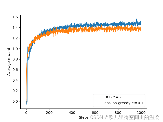
UCB算法在10臂测试平台上的平均表现，如图所示，，除了刚开始的k步随机选择尚未尝试过的动作外，在一般情况下UCB算法比ε贪心算法更好。

 

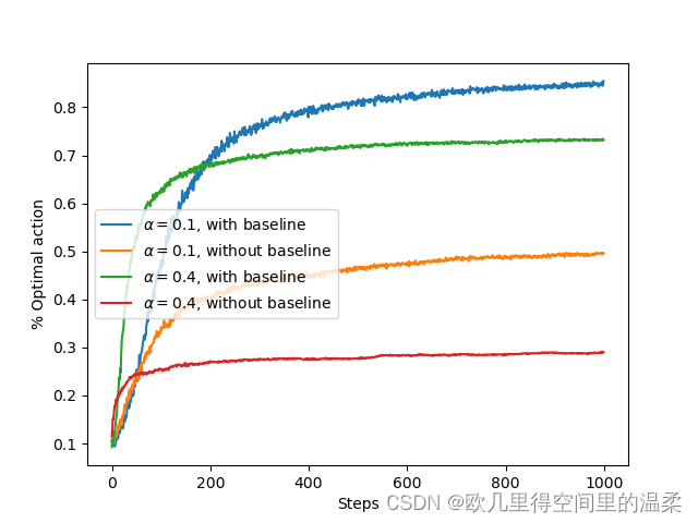
含有收益基准项和不含有收益基准项的梯度赌博算法在10臂测试平台上的平均表现。其中我们设定q*(a)接近与+4而不是0