


本文选取的是2022年五一杯数学建模b题,一道预测问题,通过可视化方法对数据进行绘制,选用随机森林模型进行预测。(只做前三问)
题目如下:
第一问第二问代码段:
import pandas as pd
from pandas.tseries.offsets import DateOffset
from statsmodels.tsa.statespace.varmax import VARMAX
from statsmodels.tsa.stattools import adfuller
import matplotlib.pyplot as plt
from statsmodels.tsa.arima.model import ARIMA
import seaborn as sns
from sklearn.ensemble import RandomForestRegressor
from sklearn.model_selection import train_test_split
from sklearn.metrics import mean_squared_error
import matplotlib
# 设置Matplotlib字体和正负号显示
matplotlib.rc('font', family='SimHei')
plt.rcParams['axes.unicode_minus'] = False # 确保负号(-)显示正常
# 加载上传的 Excel 文件
file_path = r"D:\jianmo dataset\attlater.xlsx"
xls = pd.ExcelFile(file_path)
# 获取所有 sheet 的名称
sheet_names = xls.sheet_names
sheet_names
# 读取所有工作表的数据
data_frames = {}
for sheet in sheet_names:
data_frames[sheet] = pd.read_excel(xls, sheet)
for sheet in sheet_names:
print(sheet)
for sheet in sheet_names:
print(f"Sheet Name: {sheet}")
df = data_frames[sheet] # 获取当前工作表的DataFrame
for column in df.columns:
print(f"Column Name: {column}")
print(df[column]) # 打印当前列的数据
print("-----------------------")
# 假设 data_frames 字典中包含了温度表格和产品质量表格,键分别为 '温度表格' 和 '产品质量表格'
temperature_df = data_frames['温度(temperature)']
quality_df = data_frames['产品质量(quality of the products)']
# 合并两个表格,根据时间列进行合并
merged_df = pd.merge(temperature_df, quality_df, on='时间 (Time)', how='inner')
# 输出合并后的 DataFrame
print(merged_df)
merged_file_path = "merged_data.xlsx"
merged_df['时间 (Time)'] = merged_df['时间 (Time)'].dt.strftime('%Y/%m/%d %H:%M:%S')
# 将合并后的数据写入新的Excel文件
merged_df.to_excel(merged_file_path, index=False)
# 重新读取新建的Excel文件
new_merged_df = pd.read_excel("merged_data.xlsx")
# 显示读取的数据
print(new_merged_df)
# 定义一个空的DataFrame作为存储目标
data = pd.DataFrame()
# 合并两个 DataFrame,按行合并
data = pd.concat([data, new_merged_df], ignore_index=True)
# 打印合并后的数据
print(data)
# Convert '时间 (Time)' to datetime format for better plotting
data['时间 (Time)'] = pd.to_datetime(data['时间 (Time)'])
# Setting up the figure and axes for plotting
fig, axes = plt.subplots(nrows=3, ncols=2, figsize=(14, 10), sharex=True)
fig.suptitle('Temperature and Index Time Series', fontsize=16)
# Temperature of system I
axes[0, 0].plot(data['时间 (Time)'], data['系统I温度 (Temperature of system I)'], color='tab:red')
axes[0, 0].set_title('Temperature of System I')
axes[0, 0].set_ylabel('Temperature')
# Temperature of system II
axes[0, 1].plot(data['时间 (Time)'], data['系统II温度 (Temperature of system II)'], color='tab:blue')
axes[0, 1].set_title('Temperature of System II')
axes[0, 1].set_ylabel('Temperature')
# Index A
axes[1, 0].plot(data['时间 (Time)'], data['指标A (index A)'], color='tab:green')
axes[1, 0].set_title('Index A')
axes[1, 0].set_ylabel('Index Value')
# Index B
axes[1, 1].plot(data['时间 (Time)'], data['指标B (index B)'], color='tab:orange')
axes[1, 1].set_title('Index B')
axes[1, 1].set_ylabel('Index Value')
# Index C
axes[2, 0].plot(data['时间 (Time)'], data['指标C (index C)'], color='tab:purple')
axes[2, 0].set_title('Index C')
axes[2, 0].set_ylabel('Index Value')
# Index D
axes[2, 1].plot(data['时间 (Time)'], data['指标D (index D)'], color='tab:brown')
axes[2, 1].set_title('Index D')
axes[2, 1].set_ylabel('Index Value')
# Setting up x-axis label for all
for ax in axes.flat:
ax.set_xlabel('Time')
ax.label_outer()
plt.tight_layout(rect=[0, 0.03, 1, 0.95])
plt.show()
# 重置之前的数据准备环节,排除日期时间类型的数据,并仅保留系统I和II的温度数据
# 这里我们会创建一个函数来准备输入特征和目标,排除时间列
def prepare_data_for_RF(df, target_column, n_lags):
# 创建滞后特征
df_lagged = df.copy()
for n in range(1, n_lags + 1):
df_lagged[f'{target_column} lag_{n}'] = df_lagged[target_column].shift(n)
df_lagged.dropna(inplace=True)
# 排除时间列和目标列以外的所有列,这里假设时间列命名为 '时间 (Time)'
X = df_lagged.drop(['时间 (Time)', target_column], axis=1)
y = df_lagged[target_column]
return X, y
# 以'系统I温度 (Temperature of system I)'为目标来预测
# 使用3个滞后特征作为输入
X, y = prepare_data_for_RF(data, '系统I温度 (Temperature of system I)', 3)
# 再次进行数据集分割
X_train, X_test, y_train, y_test = train_test_split(X, y, test_size=0.2, random_state=42)
# 使用随机森林模型
rf_model = RandomForestRegressor(n_estimators=100, random_state=42)
# 训练模型
rf_model.fit(X_train, y_train)
# 进行预测
predictions = rf_model.predict(X_test)
# 计算测试集上的均方误差(MSE)
mse = mean_squared_error(y_test, predictions)
mse, predictions[:5]
X = data[['系统I温度 (Temperature of system I)', '系统II温度 (Temperature of system II)']]
y_a = data['指标A (index A)']
y_b = data['指标B (index B)']
y_c = data['指标C (index C)']
y_d = data['指标D (index D)']
# 由于数据集较小,我们将使用所有数据来训练模型
# 在实际情况中,应该使用训练集和测试集来评估模型的性能
# 训练模型来预测指标A
model_a = RandomForestRegressor(n_estimators=100, random_state=42)
model_a.fit(X, y_a)
# 训练模型来预测指标B
model_b = RandomForestRegressor(n_estimators=100, random_state=42)
model_b.fit(X, y_b)
# 训练模型来预测指标C
model_c = RandomForestRegressor(n_estimators=100, random_state=42)
model_c.fit(X, y_c)
# 训练模型来预测指标D
model_d = RandomForestRegressor(n_estimators=100, random_state=42)
model_d.fit(X, y_d)
# 已知的系统I和系统II的温度值
known_temperatures = [
[1404.89, 859.77], # 第一个时间点的温度值
[1151.75, 859.77] # 第二个时间点的温度值
]
# 将已知温度值转换为DataFrame,用于预测
X_pred = pd.DataFrame(known_temperatures, columns=['系统I温度 (Temperature of system I)', '系统II温度 (Temperature of system II)'])
# 使用模型进行预测
predictions_a = model_a.predict(X_pred)
predictions_b = model_b.predict(X_pred)
predictions_c = model_c.predict(X_pred)
predictions_d = model_d.predict(X_pred)
# 创建一个空的DataFrame以存储预测结果
new_data_to_predict = pd.DataFrame()
# 添加时间列
new_data_to_predict['时间 (Time)'] = pd.to_datetime(['2022-01-24', '2022-01-24'])
# 将预测结果添加到新DataFrame中
new_data_to_predict['预测指标A (Predicted Index A)'] = predictions_a
new_data_to_predict['预测指标B (Predicted Index B)'] = predictions_b
new_data_to_predict['预测指标C (Predicted Index C)'] = predictions_c
new_data_to_predict['预测指标D (Predicted Index D)'] = predictions_d
pd.set_option('display.max_columns', None) # 显示所有列
pd.set_option('display.max_rows', None) # 显示所有行
pd.set_option('display.expand_frame_repr', False) # 禁止自动换行(避免DataFrame展示不全)
# 已知的系统I和系统II的温度值
known_temperatures = [
[1404.89, 859.77], # 第一个时间点的温度值
[1151.75, 859.77] # 第二个时间点的温度值
]
# 将已知温度值转换为DataFrame,用于预测
X_pred = pd.DataFrame(known_temperatures, columns=['系统I温度 (Temperature of system I)', '系统II温度 (Temperature of system II)'])
# 使用模型进行预测
predictions_a = model_a.predict(X_pred)
predictions_b = model_b.predict(X_pred)
predictions_c = model_c.predict(X_pred)
predictions_d = model_d.predict(X_pred)
# 创建一个空的DataFrame以存储预测结果
new_data_to_predict = pd.DataFrame()
# 添加时间列
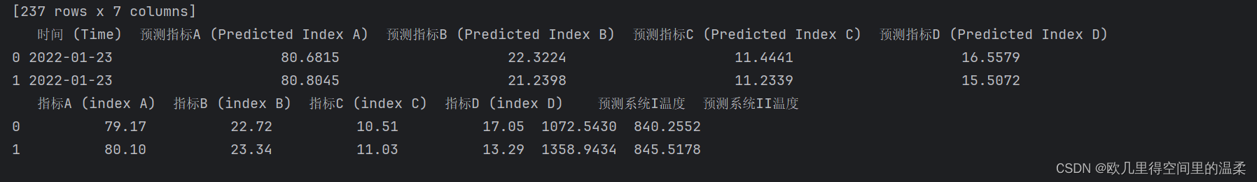
new_data_to_predict['时间 (Time)'] = pd.to_datetime(['2022-01-23', '2022-01-23'])
# 将预测结果添加到新DataFrame中
new_data_to_predict['预测指标A (Predicted Index A)'] = predictions_a
new_data_to_predict['预测指标B (Predicted Index B)'] = predictions_b
new_data_to_predict['预测指标C (Predicted Index C)'] = predictions_c
new_data_to_predict['预测指标D (Predicted Index D)'] = predictions_d
# 显示最终的预测结果DataFrame
print(new_data_to_predict)
X = data[['指标A (index A)', '指标B (index B)', '指标C (index C)', '指标D (index D)']]
y_i = data['系统I温度 (Temperature of system I)']
y_ii = data['系统II温度 (Temperature of system II)']
# 分割数据集为训练集和测试集
X_train, X_test, y_i_train, y_i_test = train_test_split(X, y_i, test_size=0.2, random_state=42)
X_train, X_test, y_ii_train, y_ii_test = train_test_split(X, y_ii, test_size=0.2, random_state=42)
# 训练模型
model_i = RandomForestRegressor(n_estimators=100, random_state=42)
model_ii = RandomForestRegressor(n_estimators=100, random_state=42)
model_i.fit(X_train, y_i_train)
model_ii.fit(X_train, y_ii_train)
# 准备新数据,即问题中给定的指标值
new_indices = {
'指标A (index A)': [79.17, 80.10],
'指标B (index B)': [22.72, 23.34],
'指标C (index C)': [10.51, 11.03],
'指标D (index D)': [17.05, 13.29]
}
new_data_to_predict = pd.DataFrame(new_indices)
# 使用模型进行预测
predicted_i_temperatures = model_i.predict(new_data_to_predict)
predicted_ii_temperatures = model_ii.predict(new_data_to_predict)
# 输出预测结果
new_data_to_predict['预测系统I温度'] = predicted_i_temperatures
new_data_to_predict['预测系统II温度'] = predicted_ii_temperatures
print(new_data_to_predict)
代码运行结果为: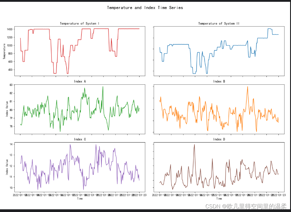
即为前两文的答案。
第三问代码:
import pandas as pd
from pandas.tseries.offsets import DateOffset
from statsmodels.tsa.statespace.varmax import VARMAX
from statsmodels.tsa.stattools import adfuller
import matplotlib.pyplot as plt
from statsmodels.tsa.arima.model import ARIMA
from sklearn.ensemble import RandomForestRegressor
from sklearn.model_selection import train_test_split
from sklearn.metrics import mean_squared_error
from sklearn.inspection import PartialDependenceDisplay
from SALib.sample import saltelli
from SALib.analyze import sobol
from sklearn.metrics import mean_squared_error
import matplotlib
import numpy as np
# 设置文件路径
file_path = r"D:\jianmo dataset\attachment2.xlsx"
# 使用ExcelFile对象处理多个工作表
xls = pd.ExcelFile(file_path)
# 获取所有工作表的名称
sheet_names = xls.sheet_names
# 读取所有工作表的数据
data_frames = {}
for sheet in sheet_names:
df = pd.read_excel(xls, sheet_name=sheet)
print(f"基本统计信息 ({sheet}):")
print(df.describe()) # 显示基本统计信息
data_frames[sheet] = df
# 特别处理温度数据表中的缺失值,删除所有包含缺失值的行
if "温度(temperature)" in data_frames:
data_frames["温度(temperature)"].dropna(inplace=True)
# 处理异常值的函数,改进为对每列分别应用
def handle_outliers(df):
"""对DataFrame的每个数值列使用IQR方法检测和处理异常值"""
for column in df.select_dtypes(include=[np.number]).columns:
Q1 = df[column].quantile(0.25)
Q3 = df[column].quantile(0.75)
IQR = Q3 - Q1
lower_bound = Q1 - 1.5 * IQR
upper_bound = Q3 + 1.5 * IQR
df[column] = df[column].clip(lower=lower_bound, upper=upper_bound)
return df
# 对每个数据表应用异常值处理
for name, df in data_frames.items():
if df.select_dtypes(include=[np.number]).empty is False: # 只对数值型列处理
data_frames[name] = handle_outliers(df.select_dtypes(include=[np.number]))
# 保存处理后的数据到新的Excel文件
output_path = r"D:\jianmo dataset\cleaned_attachment2.xlsx"
with pd.ExcelWriter(output_path) as writer:
for name, df in data_frames.items():
df.to_excel(writer, sheet_name=name, index=False)
# 输出保存成功的消息
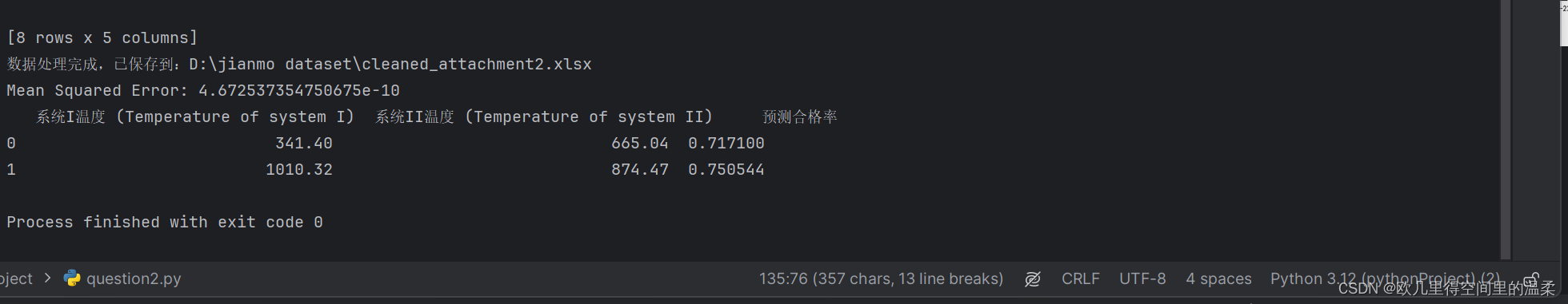
print("数据处理完成,已保存到:" + output_path)
# 加载数据
file_path = 'D:\\jianmo dataset\\cleaned_attachment2.xlsx'
data = pd.read_excel(file_path)
# 假设每天24条数据
num_complete_days = len(data) // 24
# 生成日期序列,计算日均温度
start_date = pd.Timestamp('2022-01-25')
dates = pd.date_range(start=start_date, periods=num_complete_days, freq='D')
# 计算日均值,确保只包括完整的天数的数据
daily_data = data.iloc[:num_complete_days * 24].groupby(data.index[:num_complete_days * 24] // 24).mean()
daily_data['Date'] = dates
# 生成假的合格率数据,用于演示
np.random.seed(42) # 为了结果的可重复性
daily_data['合格率'] = np.clip(0.75 + 0.005 * (daily_data['系统I温度 (Temperature of system I)'] - 1000) / 100, 0, 1)
# 准备数据
X = daily_data[['系统I温度 (Temperature of system I)', '系统II温度 (Temperature of system II)']]
y = daily_data['合格率']
# 数据划分
X_train, X_test, y_train, y_test = train_test_split(X, y, test_size=0.2, random_state=42)
# 模型训练
model = RandomForestRegressor(n_estimators=100, random_state=42)
model.fit(X_train, y_train)
# 预测和评估
y_pred = model.predict(X_test)
mse = mean_squared_error(y_test, y_pred)
print(f"Mean Squared Error: {mse}")
predict_dates = {
'系统I温度 (Temperature of system I)': [341.40, 1010.32],
'系统II温度 (Temperature of system II)': [665.04, 874.47]
}
predict_df = pd.DataFrame(predict_dates)
# 使用模型进行预测
predicted_qualification_rates = model.predict(predict_df)
# 使用模型进行预测
predicted_qualification_rates = model.predict(predict_df)
# 将预测结果添加到DataFrame中以便显示
predict_df['预测合格率'] = predicted_qualification_rates
# 显示包含预测结果的DataFrame
print(predict_df)填充数据之后得到的结果如图所示
在图中展示的是系统I和系统II的温度以及指标A、B、C、D随时间的变化。随机森林模型通常被选用来进行此类数据的预测,主要有以下几个原因:
-
处理非线性关系:
- 随机森林能很好地处理数据之间的非线性关系,而时间序列数据(如温度和指标)之间往往存在复杂的非线性关系。
-
变量之间的相互作用:
- 该模型可以自动检测特征之间的相互作用,这在处理多个变量时是非常重要的,比如系统温度如何与各指标相互作用影响产品质量。
-
不需要数据预处理:
- 随机森林对数据的分布和缩放不敏感,因此不需要像线性模型那样的数据标准化或归一化。
-
抗过拟合:
- 由于其构建多棵决策树并进行结果平均的方式,随机森林具有较强的泛化能力,不容易过拟合。
-
特征重要性:
- 随机森林能提供关于特征重要性的评估,这可以帮助我们理解哪些特征在预测产品质量时最重要。
-
灵活性:
- 随机森林可以处理各种类型的数据,包括分类和回归问题,因此非常适合于预测目标变量,无论是连续还是离散。
-
可解释性:
- 尽管不如线性模型,但随机森林模型相对于其他复杂的非线性模型(如深度学习)来说,还是具有较好的可解释性。
根据图中的数据走势,可以看出数据点之间的关系可能不是简单的线性关系。因此,选用随机森林模型来捕捉这些复杂的关系是合理的选择。随机森林通过集成多个决策树来减少预测误差,使模型更加稳健。


 1万+
1万+

 被折叠的 条评论
为什么被折叠?
被折叠的 条评论
为什么被折叠?
 到【灌水乐园】发言


