图机器学习基础知识——CS224W（08-app）

CS224W: Machine Learning with Graphs

Stanford / Winter 2021

08-app

Graph Augmentation for GNNs

Key Idea: Raw input graph ≠ computational graph

Graph Augmentation: 输入数据不一定就是计算时的计算图，可以对图在结构或特征上进行augment定义新的computation graph以便于加速计算或其他目的

• 之前讨论的模型架构的假设一直都是：Raw input graph = computational graph，即训练时不对输入的图结构进行改动

• Reason for breaking this assumption

  • Features

    • The input graph lacks features (输入的图数据可能缺乏一些特征)

  • Graph Structure

    • The graph is too sparse ➡ inefficient message passing (图太稀疏➡消息传递效率低)

    • The graph is too dense ➡ message passing is too costly (图太密集➡消息传递代价高)

    • The graph is too large ➡ cannot fit the computational graph into a GPU (图太大➡GPU Memory不够用)

Graph Feature Augmentation

Graph Feature Augmentation

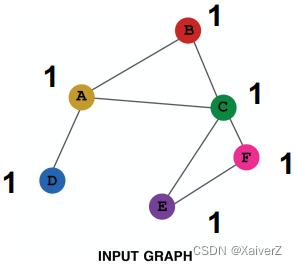
• Case-1: Input graph does not have node features (输入图节点没有特征，也就是只有图结构的信息)

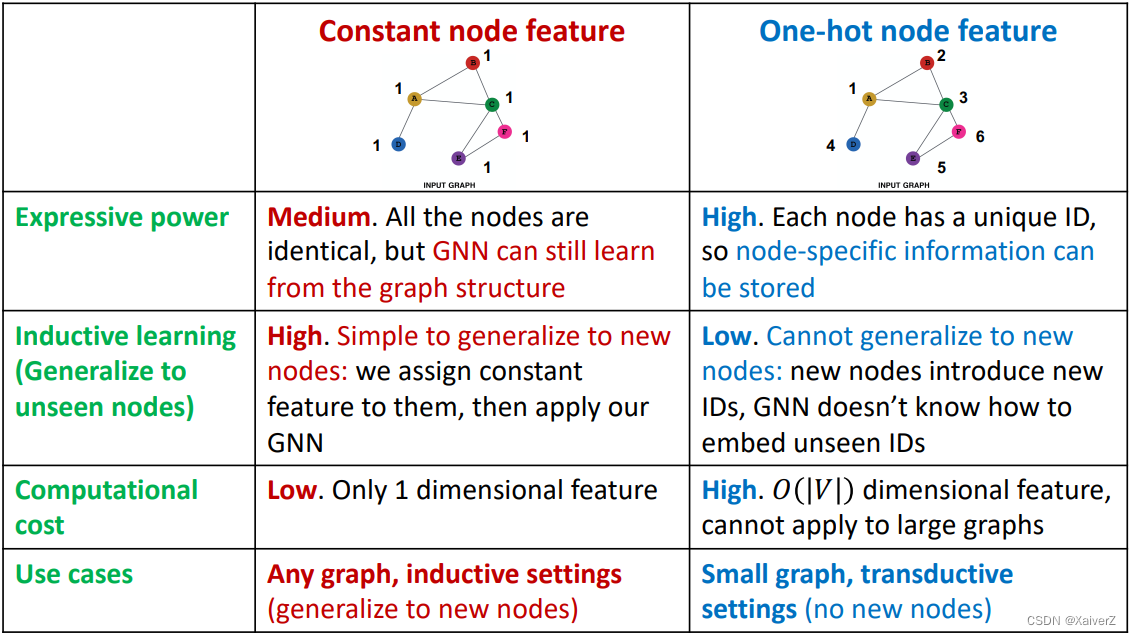
  • Assign constant value to nodes (给节点赋常数值作为初始特征)

    

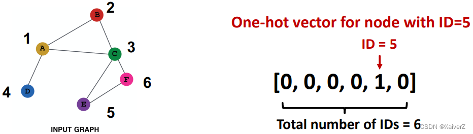
  • Assign unique IDs to nodes (给每个节点一个唯一的ID，而后转成one-hot vector作为初始特征)

    

  

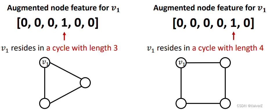
• Case-2: Certain structures are hard to learn by GNN (GNN很难学到某些特定的图结构)

  • Example: Cycle count feature. Can GNN learn the length of a cycle that $v_1$ resides in? Unfortunately, no

    

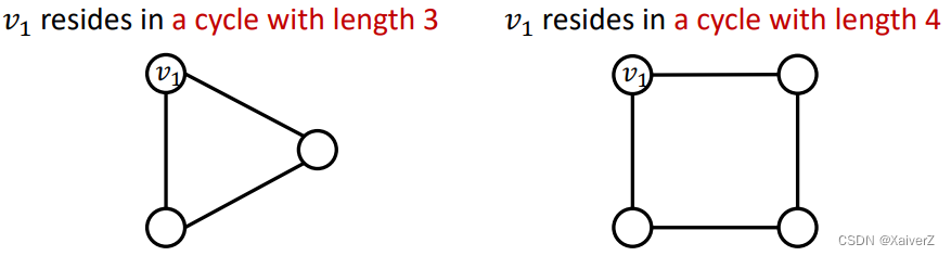
    • $v_1$ cannot differentiate which graph it resides in because all the nodes in the graph have degree of 2. The computational graphs will be the same binary tree

    

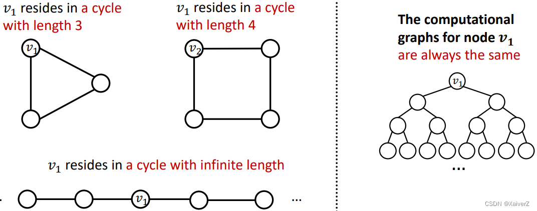
    • Solution: 额外加入cycle count作为节点的增强特征

    

  • Other commonly used augmented features

    • Node degree

    • Clustering coefficient

    • PageRank

    • Centrality

    • …Any feature introduced in lecture 2 can be used

Graph Structure Augmentation

Graph Structure Augmentation

• The graph is too sparse ➡ Add virtual nodes/edges (虚拟节点/边)

  • Add virtual edges (加虚拟边)

    • Connect 2-hop neighbors via virtual edges (连接自身与间隔两跳的邻居)

    • 矩阵形式实现：

      $$A+A^2$$

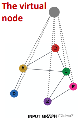
  • Add virtual nodes (加虚拟节点)

    • The virtual node will connect to all the nodes in the graph (虚拟点连接图中所有节点)

    • 假设在一个稀疏图中，两个节点之间的最短路径为10，这两个节点之间的消息传递就比较低效，要经过10-hop才能交互。当我们用一个虚拟节点连接图中所有节点时，图中所有两两节点之间的最短距离都变为了2 (Node A - Virtual Node - Node B)，极大提升了消息传递效率

    

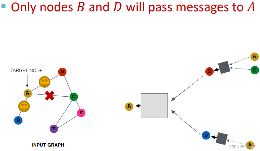
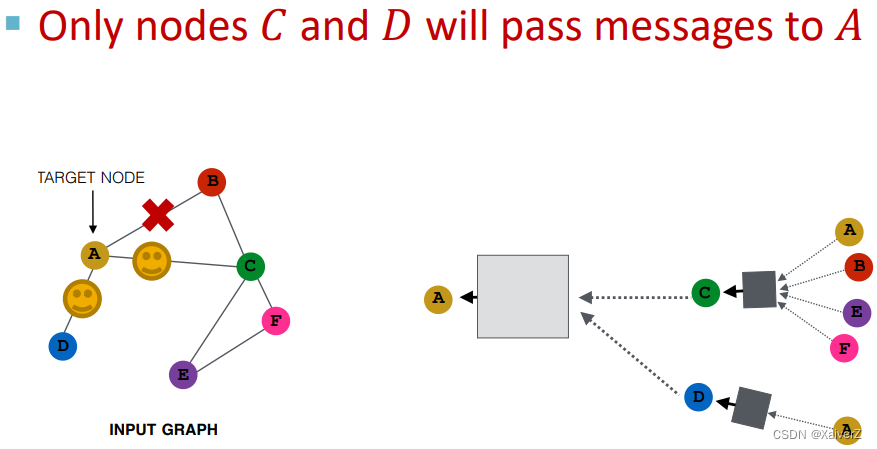
• The graph is too dense ➡ Sample neighbors when doing message passing (消息传递邻居采样)

  • 在某一层中，随机采样一些邻居进行消息传递

    

  • 在下一层，可以随机采样另一些不同的邻居进行消息传递

    

  • 使用这种方式，embedding与使用全部邻居计算相差不大，同时极大减少计算开销

• The graph is too large ➡ Sample subgraphs to compute embeddings (采样子图计算embeddings)

Prediction with GNNs

Prediction Heads: Node-level

Prediction Heads: Edge-level

Make prediction using pairs of node embeddings

• Suppose we want to make k-way prediction

$${\hat{\mathbf{y}}}_{\mathbf{uv}}={\mathrm{Head}}_{\mathrm{edg}e}\left({\mathbf{h}}_u^{(L)},{\mathbf{h}}_v^{(L)}\right)$$

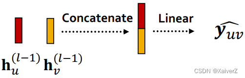
• Options for Head ${}_{\text{edge }}\left({\mathbf{h}}_u^{(L)},{\mathbf{h}}_v^{(L)}\right)$

  • Concatenation + Linear

    

  • Dot product

    $${\hat{\mathbf{y}}}_{\mathbf{u}\mathbf{v}}={\left({\mathbf{h}}_u^{(L)}\right)}^T{\mathbf{h}}_v^{(L)}$$
    该式只适用于二分类，即预测边存不存在（因为点积后为一个值）

    $$\begin{array}{c}{\hat{y}}_{uv}^{(1)}={\left({\mathbf{h}}_u^{(L)}\right)}^T{\mathbf{W}}^{(1)}{\mathbf{h}}_v^{(L)}\\ \dots \\ {\hat{y}}_{uv}^{(k)}={\left({\mathbf{h}}_u^{(-)}\right)}^T{\mathbf{W}}^{(k)}{\mathbf{h}}_v^{(L)}\\ {\hat{\mathbf{y}}}_{uv}=\mathrm{Concat}\left({\hat{y}}_{uv}^{(1)},\dots ,{\hat{y}}_{uv}^{(k)}\right)\in {\mathbb{R}}^k\end{array}$$
    该式应用了multi-head attention，能适用于多分类

Prediction Heads: Graph-level

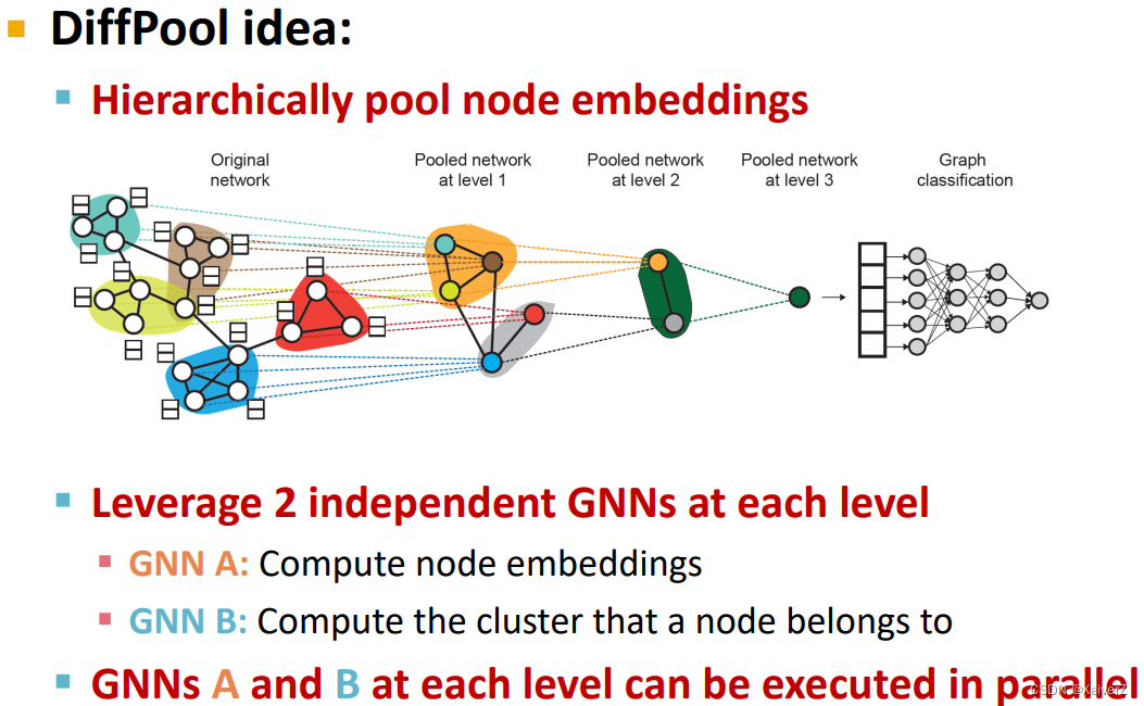
Paper : Hierarchical Graph Representation Learning with Differentiable Pooling

Make prediction using all the node embeddings in our graph

• Suppose we want to make k-way prediction

$${\hat{\mathbf{y}}}_G={\mathrm{Head}}_{\mathrm{graph}}\left(\left\{{\mathbf{h}}_v^{(L)}\in {\mathbb{R}}^d,\forall v\in G\right\}\right)$$

• Options for ${\mathrm{Head}}_{\mathrm{graph}}\left(\left\{{\mathbf{h}}_v^{(L)}\in {\mathbb{R}}^d,\forall v\in G\right\}\right)$

  • Global mean pooling

    $${\hat{\mathbf{y}}}_G=\mathrm{Mean}\left(\left\{{\mathbf{h}}_v^{(L)}\in {\mathbb{R}}^d,\forall v\in G\right\}\right)$$

  • Global max pooling

    $${\hat{\mathbf{y}}}_G=\mathrm{Max}\left(\left\{{\mathbf{h}}_v^{(L)}\in {\mathbb{R}}^d,\forall v\in G\right\}\right)$$

  • Global sum pooling

    $${\hat{\mathbf{y}}}_G=\mathrm{Sum}\left(\left\{{\mathbf{h}}_v^{(L)}\in {\mathbb{R}}^d,\forall v\in G\right\}\right)$$

• Issue of Global Pooling

  • Global pooling over a (large) graph will lose information

  • Example: we use 1-dim node embeddings

    • Node embeddings for G 1 : { − 1 , − 2 , 0 , 1 , 2 } G_{1}:\{-1,-2,0,1,2\} G1​:{−1,−2,0,1,2}

    • Node embeddings for G 2 : { − 10 , − 20 , 0 , 10 , 20 } G_{2}:\{-10,-20,0,10,20\} G2​:{−10,−20,0,10,20}

    • 非常明显两个图有非常不同的node embedding，它们的结构应该不同

    • 但如果我们用global sum pooling

      • Prediction for G 1 : y ^ G = Sum ⁡ ( { − 1 , − 2 , 0 , 1 , 2 } ) = 0 G_{1}: \hat{y}_{G}=\operatorname{Sum}(\{-1,-2,0,1,2\})=0 G1​:y^​G​=Sum({−1,−2,0,1,2})=0

      • Prediction for G 2 : y ^ G = Sum ⁡ ( { − 10 , − 20 , 0 , 10 , 20 } ) = 0 G_{2}: \hat{y}_{G}=\operatorname{Sum}(\{-10,-20,0,10,20\})=0 G2​:y^​G​=Sum({−10,−20,0,10,20})=0

    • 无法区分两图！

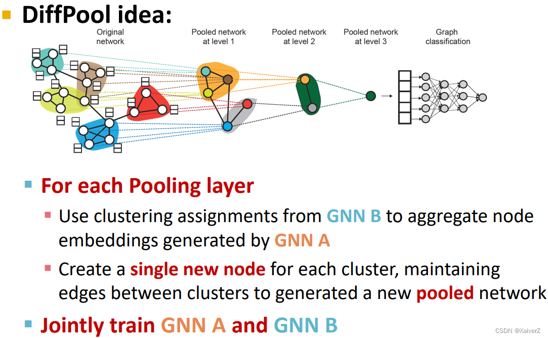
• Hierarchical Global Pooling

  • Aggregate all the node embeddings hierarchically

  • 使用$\mathrm{ReLU}(\mathrm{Sum}(\cdot ))$来进行aggregate: 先对前两个节点聚合，再对后三个节点聚合

    • G 1 : { − 1 , − 2 , 0 , 1 , 2 } G_{1}:\{-1,-2,0,1,2\} G1​:{−1,−2,0,1,2}

      y ^ a = ReLU ⁡ ( Sum ⁡ ( { − 1 , − 2 } ) ) = 0 \hat{y}_{a}=\operatorname{ReLU}(\operatorname{Sum}(\{-1,-2\}))=0 y^​a​=ReLU(Sum({−1,−2}))=0

      y ^ b = ReLU ⁡ ( Sum ⁡ ( { 0 , 1 , 2 } ) ) = 3 \hat{y}_{b}=\operatorname{ReLU}(\operatorname{Sum}(\{0,1,2\}))=3 y^​b​=ReLU(Sum({0,1,2}))=3

      y ^ G = ReLU ⁡ ( Sum ⁡ ( { y a , y b } ) ) = 3 \hat{y}_{G}=\operatorname{ReLU}\left(\operatorname{Sum}\left(\left\{y_{a}, y_{b}\right\}\right)\right)=3 y^​G​=ReLU(Sum({ya​,yb​}))=3

    • G 2 : { − 10 , − 20 , 0 , 10 , 20 } G_{2}:\{-10,-20,0,10,20\} G2​:{−10,−20,0,10,20}

      y ^ a = ReLU ⁡ ( Sum ⁡ ( { − 10 , − 20 } ) ) = 0 \hat{y}_{a}=\operatorname{ReLU}(\operatorname{Sum}(\{-10,-20\}))=0 y^​a​=ReLU(Sum({−10,−20}))=0

      y ^ b = ReLU ⁡ ( Sum ⁡ ( { 0 , 10 , 20 } ) ) = 30 \hat{y}_{b}=\operatorname{ReLU}(\operatorname{Sum}(\{0,10,20\}))=30 y^​b​=ReLU(Sum({0,10,20}))=30

      y ^ G = ReLU ⁡ ( Sum ⁡ ( { y a , y b } ) ) = 30 \hat{y}_{G}=\operatorname{ReLU}\left(\operatorname{Sum}\left(\left\{y_{a}, y_{b}\right\}\right)\right)=30 y^​G​=ReLU(Sum({ya​,yb​}))=30

  • 使用层次池化从而可以区分出两图

• Hierarchical Pooling

  

  

Dataset Split: Fixed / Random Split

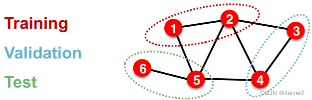
Node Classification

• 每个样本（节点）之间不是独立的，由于有连边，所以会互相影响

  

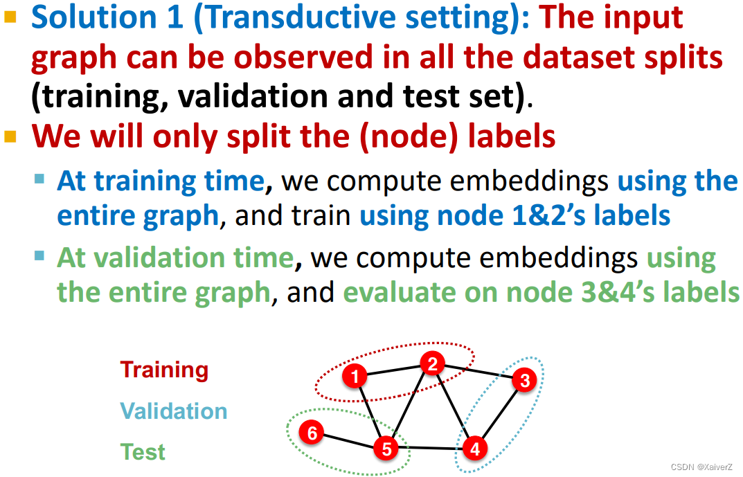
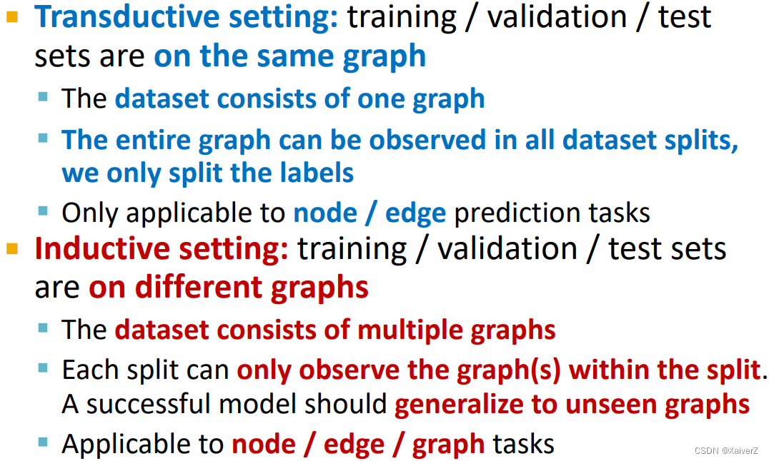
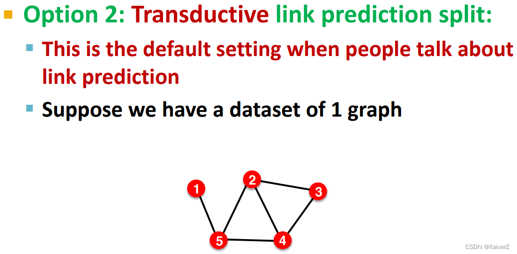
• Solution-1: Transductive setting

  

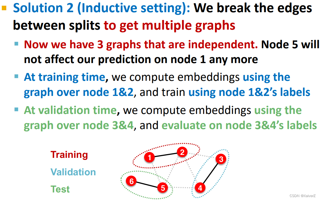
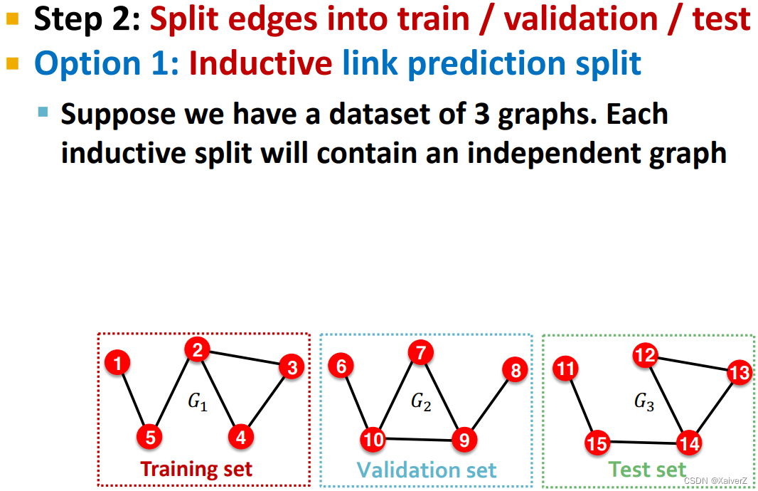
• Solution-2: Inductive setting

  

• Transductive / Inductive Settings

  

Graph Classification

• 图分类没有类似于节点分类那种数据不独立的问题

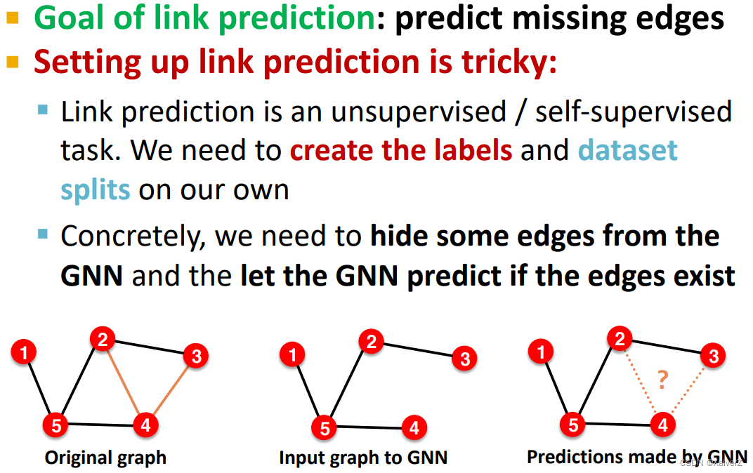
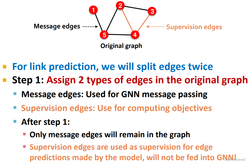
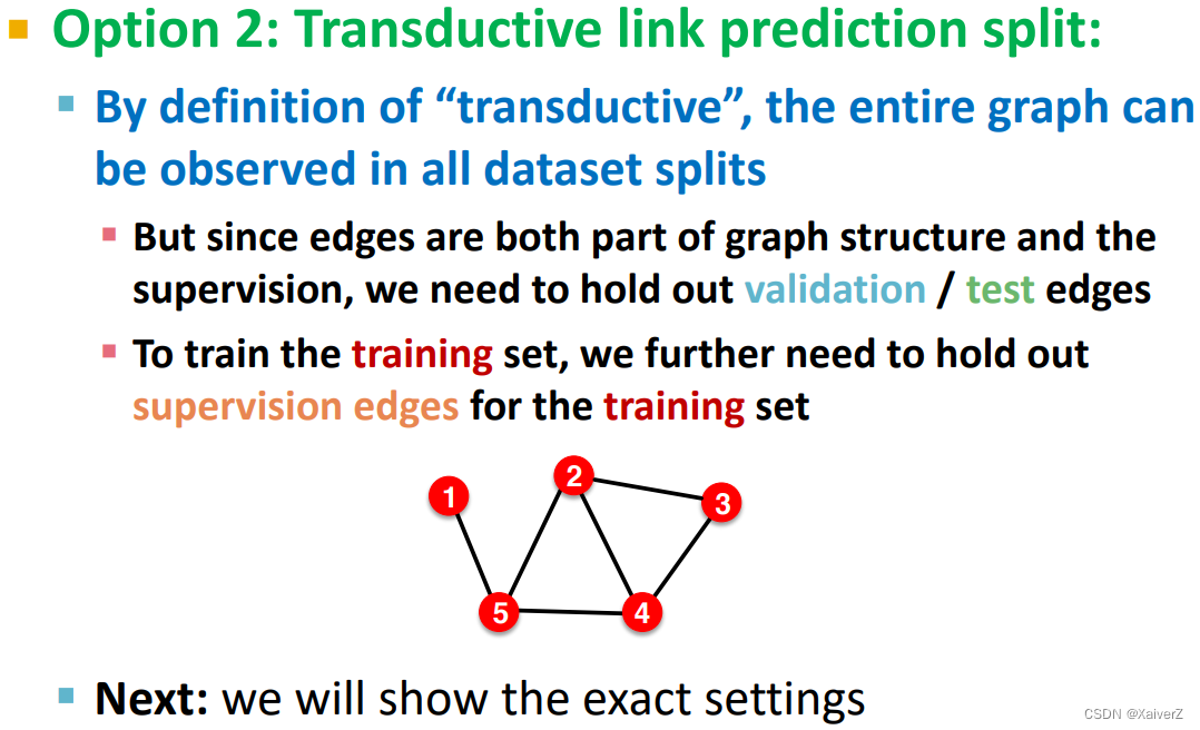
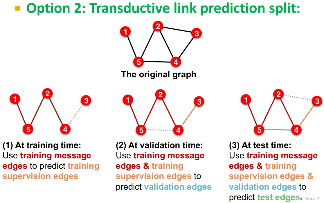
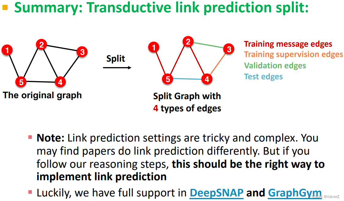
Link Prediction