《机器学习实战》笔记1 - KNN手写数字

简述KNN

KNN原理

通过计算特征向量之间距离的方法，找出距离待测试的向量最小的k个训练样本，统计他们的标签，标签数量最多的一个就是我们预测的结果。距离的计算可以自己定义，如欧式距离，曼哈顿距离哪个效果好就用哪个。k的选取也会对结果产生较大的影响，调整k值（所谓调参）以获得最好的效果。

优点

1、算法简单，易于实现
2、可以作分类，也可以做回归
3、对异常值不敏感，准确度高，对数据没有假定

缺点

1、时间复杂度、空间复杂度高。取决于“训练”的样本数量
2、不像是所谓机器学习，因为它没有训练模型的过程。

---

涉及到的python知识点

1、np.tile()广播

功能：在KNN中计算距离时，将当前特征向量广播到整个数据大小，以便利用python特性直接计算。
参考 https://blog.csdn.net/qq_18433441/article/details/54897250

2、os.listdir() 获取目录文件

功能：获取某一目录下所有文件名，可用来遍历文件夹，读取数据

3、open(filename, ‘r’) 打开文件

功能：可以打开txt文件，获取到字符串信息，用split()或replace()等方法对文本进行处理。

4、argsort()

功能：获取排序好的索引下标，可用来做递增或递减的部分遍历

5、python字典添加元素的方法

classCount[one_label] = classCount.get(one_label, 0) + 1
如果没有one_label这个key，就置0，否则读取原来的value，然后+1.

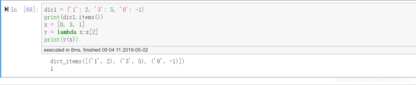
6、python字典按value排序

sortedClassCount = sorted(classCount.items(), key = lambda x:x[1], reverse=True)
三个参数默认是迭代的对象、排序按哪个值排序，是否反转（默认为升序）
按键排序也可以这样实现

7、混淆矩阵

混淆矩阵是什么可以百度，它对分析数据的预测结果很有帮助。如图是一个手写数字识别的混淆矩阵，它把十个数字预测成了什么和他们实际是什么直观地展示了出来。

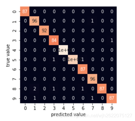
代码：利用sklearn封装的函数得出混淆矩阵，并用seaborn作图

# 绘制混淆矩阵
def sklearn_confusion_matrix(ytest, ymodel):
    from sklearn.metrics import confusion_matrix
    import seaborn as sns
    import matplotlib.pyplot as plt
    
    mat = confusion_matrix(ytest, ymodel)
    print(mat)
    sns.heatmap(mat, square=True, annot=True, cbar=False)
    plt.xlabel('predicted value')
    plt.ylabel('true value')

sklearn_confusion_matrix(test_labels, result)

8、recall、precision、F-Measure

这篇博客讲的非常好非常详细
https://www.cnblogs.com/Zhi-Z/p/8728168.html

这些概念似乎是相对于二分类问题的，所以我们这个问题（手写数字识别）是无法得出这些统计学概念的，但不妨碍我们学习。

图片来源：https://www.cnblogs.com/Zhi-Z/p/8728168.html

一个代码示例

def get_precision_recall_f1(trues, predicts):
    TP = TN = FP = FN = 0
    precisioin = recall = f1 = 0
    for i in range(len(trues)):
        if trues[i] == 1 and predicts[i] == 1:
            TP += 1
        elif trues[i] == 0 and predicts[i] == 0:
            TN += 1
        elif trues[i] == 1 and predicts[i] == 0:
            FP += 1
        elif trues[i] == 0 and predicts[i] == 1:
            FN += 1
    precision = TP / (TP + FP)
    recall = TP / (TP + FN)
    f1 = 2*precision*recall / (precision + recall)
    return precision, recall, f1

trues = [1, 1, 1, 1, 0, 0, 0, 1, 0, 1, 1, 1, 1, 0, 1, 1, 1, 0, 1, 1]
predicts = [1, 1, 0, 1, 0, 0, 1, 1, 0, 1, 1, 1, 0, 0, 1, 1, 0, 0, 1, 1]
sklearn_confusion_matrix(trues, predicts)
    
precision, recall, f1 = get_precision_recall_f1(trues, predicts)
print("precision = {}, recall = {}, f1 = {}".format(precision, recall, f1))

输出结果

---

完整KNN示例代码

由于我是在jupyter notebook上写的代码，所以直接把它下载成py文件，看上去格式不怎么好。代码也无法直接运行，仅供参考。

#!/usr/bin/env python
# coding: utf-8
# In[52]:


import numpy as np
import matplotlib.pyplot as plt
import pandas as pd
import os
get_ipython().run_line_magic('matplotlib', 'inline')


# In[53]:


def getFileArray(filename):
    file_array = []
    labels = []
    train_files = os.listdir(filename)
    for each in train_files:
        labels.append(each[0])
        tmp_file = open(filename + '/' + each, 'r')
        contents = tmp_file.read().replace('\n', '')
        tmp = []
        for i in range(1024):
            tmp.append(int(contents[i]))
        file_array.append(tmp)
    return np.array(file_array), np.array(labels)


# In[54]:


digits_matrix, digit_labels = getFileArray('./digits/trainingDigits')
test_x, test_labels = getFileArray('./digits/testDigits')


# In[55]:


def knn(xtest, data, label, k): # xtest为测试的特征向量，data、label为“训练”数据集，k为设定的阈值
#     print(xtest.shape)
#     print(label.shape)
    exp_xtest = np.tile(xtest, (len(label), 1)) - data
    sq_diff = exp_xtest**2
    sum_diff = sq_diff.sum(axis=1)
    distance = sum_diff**0.5
#     print(distance)
    sort_index = distance.argsort()
    classCount = {}
    for i in range(k):
        one_label = label[sort_index[i]]
        classCount[one_label] = classCount.get(one_label, 0) + 1
    sortedClassCount = sorted(classCount.items(), key = lambda x:x[1], reverse=True)
#     print(sortedClassCount)
    return sortedClassCount[0][0]


# In[56]:


result = []
for i in range(len(test_x)):
    result.append(knn(test_x[i], digits_matrix, digit_labels, 3))


# In[57]:


print(test_labels)
print(len(test_labels))
print(len(result))


# In[51]:


# print(result)
wrong = 0
right = 0
for i in range(len(result)):
    if result[i] != test_labels[i]:
        wrong += 1
    else:
        right += 1
print("wrong = {} right = {}".format(wrong, right))
print("accurate: {}".format(right / (wrong + right)))
print("wrong rate: {}".format(wrong / (wrong + right)))


# In[70]:


# 绘制混淆矩阵
def sklearn_confusion_matrix(ytest, ymodel):
    from sklearn.metrics import confusion_matrix
    import seaborn as sns
    import matplotlib.pyplot as plt
    
    mat = confusion_matrix(ytest, ymodel)
    print(mat)
    sns.heatmap(mat, square=True, annot=True, cbar=False)
    plt.xlabel('predicted value')
    plt.ylabel('true value')

sklearn_confusion_matrix(test_labels, result)


# In[68]:


dic1 = {'1': 2, '3': 5, '0': -1}
print(dic1.items())
x = [0, 3, 1]
y = lambda x:x[2]
print(y(x))


# In[76]:





# In[92]:


def get_precision_recall_f1(trues, predicts):
    TP = TN = FP = FN = 0
    precisioin = recall = f1 = 0
    for i in range(len(trues)):
        if trues[i] == 1 and predicts[i] == 1:
            TP += 1
        elif trues[i] == 0 and predicts[i] == 0:
            TN += 1
        elif trues[i] == 1 and predicts[i] == 0:
            FP += 1
        elif trues[i] == 0 and predicts[i] == 1:
            FN += 1
    precision = TP / (TP + FP)
    recall = TP / (TP + FN)
    f1 = 2*precision*recall / (precision + recall)
    return precision, recall, f1

trues = [1, 1, 1, 1, 0, 0, 0, 1, 0, 1, 1, 1, 1, 0, 1, 1, 1, 0, 1, 1]
predicts = [1, 1, 0, 1, 0, 0, 1, 1, 0, 1, 1, 1, 0, 0, 1, 1, 0, 0, 1, 1]
sklearn_confusion_matrix(trues, predicts)
    
precision, recall, f1 = get_precision_recall_f1(trues, predicts)
print("precision = {}, recall = {}, f1 = {}".format(precision, recall, f1))