


Tune-A-Video是一个Video Editing任务很好的Baseline, 后续工作例如Control Video都是在这个工作的基础上做的. 本次我们详细阅读一下Tune-A-Video代码中的关键细节, 以及做简单的复现.
关于Video Diffusion模型请参见笔记https://blog.csdn.net/wjpwjpwjp0831/article/details/141689348
代码地址: https://github.com/showlab/Tune-A-Video
0. 模型简要总结
Tune-A-Video通过One-shot的方式, 也就是, 需要对每个你希望编辑的视频, 都需要训练一次. 训练过程只需要待编辑的视频, 不需要其他的, 因为相关的world knowledge是由预训练的Stable Diffusion提供的.
既然是视频生成, 那就必须要约束生成帧的时间一致性. 因此就通过重新设计注意力机制的形式让temporal之间也进行注意力计算, 从而维持一致性. 模型的总框图如下:
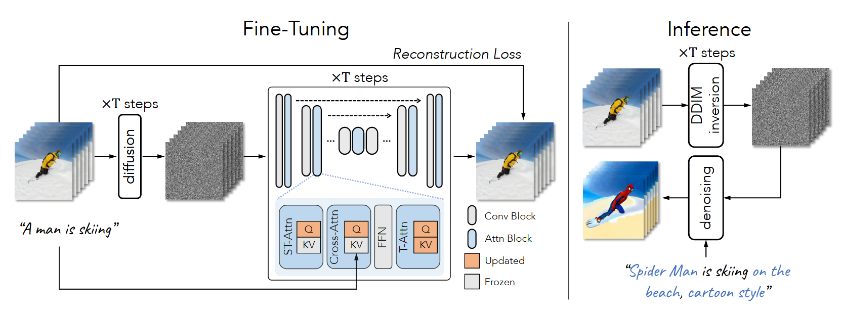
下面通过数据读取, 模型细节, 训练过程, 推理过程四部分对代码进行解读
1. 数据读取
由于是one-shot, 因此每次读入一个视频和若干要训练的prompt. 这部分代码比较简单, 这是Dataset类:
	def __getitem__(self, index):
        # load and sample video frames
        vr = decord.VideoReader(self.video_path, width=self.width, height=self.height)
        sample_index = list(range(self.sample_start_idx, len(vr), self.sample_frame_rate))[:self.n_sample_frames]
        video = vr.get_batch(sample_index)
        video = rearrange(video, "f h w c -> f c h w")  # f 帧数 c h w 图像维度

        example = {
            "pixel_values": (video / 127.5 - 1.0),  # 归一化到[-1, 1], 注意和常见的归一化到[0, 1]不同
            "prompt_ids": self.prompt_ids  # None
        }

        return example
2. 模型细节
我们以基于Stable Diffusion的Tune-A-Video为例. 首先, 基本组成部分有:
- 加噪的Scheduler,
- 去噪的Scheduler,
- 用于文本的Tokenizer,
- 用于进一步提取文本特征的text encoder,
- 将latent和RGB域互相映射的VAE encoder与decoder,
- 以及用于去噪预测的UNet.
加载模型的代码如下:
	# Load scheduler, tokenizer and models.
    noise_scheduler = DDPMScheduler.from_pretrained(pretrained_model_path, subfolder="scheduler")
    tokenizer = CLIPTokenizer.from_pretrained(pretrained_model_path, subfolder="tokenizer")
    text_encoder = CLIPTextModel.from_pretrained(pretrained_model_path, subfolder="text_encoder")
    vae = AutoencoderKL.from_pretrained(pretrained_model_path, subfolder="vae")
    unet = UNet3DConditionModel.from_pretrained_2d(pretrained_model_path, subfolder="unet")  # 从image diffusion的2D Unet中加载预训练权重
其中, UNet3DConditionModel是本文的主要贡献, 我们先看加载权重的部分:
	@classmethod
    def from_pretrained_2d(cls, pretrained_model_path, subfolder=None):
        if subfolder is not None:
            pretrained_model_path = os.path.join(pretrained_model_path, subfolder)

		# 读取模型的config文件 diffusers库是通过config文件储存模型init参数的
        config_file = os.path.join(pretrained_model_path, 'config.json')
        if not os.path.isfile(config_file):
            raise RuntimeError(f"{config_file} does not exist")
        with open(config_file, "r") as f:
            config = json.load(f)

        # 需要按照本次采用的3D Unet修改一些参数
        config["_class_name"] = cls.__name__  # 类名
        config["down_block_types"] = [  # 下采样和上采样的block需要更改 这也是模型主要修改的地方
            "CrossAttnDownBlock3D",  # 图中的ST-Attention, Cross Attention和T-Attention在这里
            "CrossAttnDownBlock3D",
            "CrossAttnDownBlock3D",
            "DownBlock3D"
        ]
        config["up_block_types"] = [
            "UpBlock3D",
            "CrossAttnUpBlock3D",
            "CrossAttnUpBlock3D",
            "CrossAttnUpBlock3D"
        ]

        from diffusers.utils import WEIGHTS_NAME  # 加载权重, 注意WEIGHTS_NAME是固定的名称, 是.bin
        # 文件, 如果需要加载safetensors需要更改, 并不能采用torch.load, 而是safetensors.torch.load
        model = cls.from_config(config)
        model_file = os.path.join(pretrained_model_path, WEIGHTS_NAME)
        if not os.path.isfile(model_file):
            raise RuntimeError(f"{model_file} does not exist")
        state_dict = torch.load(model_file, map_location="cpu")
        for k, v in model.state_dict().items():
            if '_temp.' in k:
                state_dict.update({k: v})
        model.load_state_dict(state_dict)

        return model
下面我们按照数据流的顺序, 逐层拆分该3D UNet.
2.1 输入
在前向传播过程中, 输入为:
sample: 加噪的latent, shape是(bs, c, f, h, w), 默认为(1, 4, 8, 512, 512), 其中c是4的原因是UNet的输入为VAE编码出的经过加噪后的latent, 而经过VAE编码后维度不是RGB的3, 而是4.timestep: 当前的时间步: 是作为噪声预测模型输入参数之一, 是一个Tensor, 从randint生成而来encoder_hidden_states: 这是文本的特征, 由text encoder生成
代码如下:
def forward(
        self,
        sample: torch.FloatTensor,
        timestep: Union[torch.Tensor, float, int],
        encoder_hidden_states: torch.Tensor,
        class_labels: Optional[torch.Tensor] = None,
        attention_mask: Optional[torch.Tensor] = None,
        return_dict: bool = True,
    ) -> Union[UNet3DConditionOutput, Tuple]:
我们首先需要判断, 当前输入的sample的size是否可以被上下采样倍数整除. 比如, 如果这个UNet有4个上下采样层, 那么sample的size(h和w)就必须是16的倍数. 否则的话, 我们需要强制UNet的上采样输出大小:
		default_overall_up_factor = 2**self.num_upsamplers

        # upsample size should be forwarded when sample is not a multiple of `default_overall_up_factor`
        forward_upsample_size = False
        upsample_size = None

        if any(s % default_overall_up_factor != 0 for s in sample.shape[-2:]):
            logger.info("Forward upsample size to force interpolation output size.")
            forward_upsample_size = True
forward_upsample_size会在上采样的时候用到, 用于是否强制输出大小.
2.2 对timestep进行位置编码
下面对timesteps进行embedding. 为了让模型知道当前的去噪进度, 时间步 t 需要作为输入之一. 然而, 直接将 t 作为标量输入并不能有效传递时间序列信息, 因此, 通常会对 t 进行位置编码:
P E ( t , 2 i ) = sin ( t / 1 e 4 2 i / d ) , P E ( t , 2 i + 1 ) = cos ( t / 1 e 4 2 i / d ) PE(t, 2i) = \sin (t/1e4^{2i/d}), PE(t, 2i+1) = \cos (t/1e4^{2i/d}) PE(t,2i)=sin(t/1e42i/d),PE(t,2i+1)=cos(t/1e42i/d)
这样就把一个标量
t
t
t映射到了维度为
d
d
d的向量, 向量的每一维度包含不同频率的正弦或余弦值. 这里直接用diffusers库中的Timestep进行编码:
		self.time_proj = Timesteps(block_out_channels[0], flip_sin_to_cos, freq_shift)
		# 输入: 要编码的维度, 是否将sin和cos互换(默认为true, 互换后embedding中是先cos后sin, 可能和前面介绍的sin cos交错不一样), 以及维度间频率的差别, 默认为0
		# block_out_channels = [320, 640, 1280, 1280], 表示UNet的下采样过程有四个block, 每个block的输出维度分别为320, 640, 1280, 1280
        timestep_input_dim = block_out_channels[0]

		# 位置编码后, 还需要用几个MLP进一步提取时间特征 time_embed_dim = block_out_channels[0] * 4
        self.time_embedding = TimestepEmbedding(timestep_input_dim, time_embed_dim)
在forward中, 执行时间编码:
		# broadcast to batch dimension in a way that's compatible with ONNX/Core ML
        timesteps = timesteps.expand(sample.shape[0])  # expand相当于扩展维度, 从(1, )扩展到(bs, 1)

        t_emb = self.time_proj(timesteps)

        # timesteps does not contain any weights and will always return f32 tensors
        # but time_embedding might actually be running in fp16. so we need to cast here.
        # there might be better ways to encapsulate this.
        t_emb = t_emb.to(dtype=self.dtype)
        emb = self.time_embedding(t_emb)
2.3 维度初始映射
接下来, 我们首先对sample进行卷积, 将其输出维度变为block_out_channels[0]. 因为我们输入的是多了一个视频帧数维的5维张量, 因此将其转换为2D卷积, 就需要先把f和bs合到一起:
# 定义
self.conv_in = InflatedConv3d(in_channels, block_out_channels[0], kernel_size=3, padding=(1, 1))
其中
class InflatedConv3d(nn.Conv2d):
    def forward(self, x):
        video_length = x.shape[2]

        x = rearrange(x, "b c f h w -> (b f) c h w")  # 把f和bs合到一起
        x = super().forward(x)  # 2D卷积
        x = rearrange(x, "(b f) c h w -> b c f h w", f=video_length)  # 恢复

        return x
在forward中:
sample = self.conv_in(sample) # 这时sample的维度从(1, 4, 8, 512, 512) 变为 (1, 320, 8, 256, 256)
2.4 降采样
随后是经典的降采样和升采样环节. 在降采样中, 经过的block分别为"CrossAttnDownBlock3D", CrossAttnDownBlock3D", "CrossAttnDownBlock3D", "DownBlock3D". 因此前三个是有交叉注意力的, 其需要和文本特征融合, 此外也是本文提出的时空Attention的地方. 后一个是普通的降采样.
在前向传播时, 分别经过这些层的传播过程即可. 对于不同的层有不同的输入, 因此有一个属性判断.
		# down
        down_block_res_samples = (sample,)  # 用于记录中间状态输出, 在上采样层还需要concat
        for downsample_block in self.down_blocks:
            if hasattr(downsample_block, "has_cross_attention") and downsample_block.has_cross_attention:
                sample, res_samples = downsample_block(
                    hidden_states=sample,
                    temb=emb,  # 时间步embedding
                    encoder_hidden_states=encoder_hidden_states,  # 文本embedding
                    attention_mask=attention_mask,  # 默认为None
                )
            else:
                sample, res_samples = downsample_block(hidden_states=sample, temb=emb)

            down_block_res_samples += res_samples
下面分别看这两种Block.
2.4.1 CrossAttnDownBlock3D
每个UNet block整体的结构是, 分若干个层, 每个层的输入输出维度是一样的(第一层除外). 在每个层中, 都是一个ResNet block(这里是ResNet 3D)后面跟一个注意力机制的block(Transformer block).
输入参数如下:
class CrossAttnDownBlock3D(nn.Module):
    def __init__(
        self,
        in_channels: int,  # 这个block的输入维度, block之间的输入输出遵循[320, 640, 1280, 1280], 例如如果这是第一个block, in channel就是320
        out_channels: int,  # 如果是第一个block, out就是640
        temb_channels: int,  # 前面提到的, 4 * block_out_channels[0] = 1280
        dropout: float = 0.0,
        num_layers: int = 1,  # 采用的是2
        resnet_eps: float = 1e-6,
        resnet_time_scale_shift: str = "default",
        resnet_act_fn: str = "swish",
        resnet_groups: int = 32,
        resnet_pre_norm: bool = True,
        attn_num_head_channels=1,  # 默认为8, 做8头注意力机制
        cross_attention_dim=1280,
        output_scale_factor=1.0,
        downsample_padding=1,  # 默认为1, kernel size3, stride 1, padding 1为2倍下采样
        add_downsample=True,  # 在最后下采样一次, 为True
        dual_cross_attention=False,  # 默认False
        use_linear_projection=False,  # 默认为False, 这是控制在注意力block中在计算注意力之前是用线性映射还是2D卷积
        only_cross_attention=False,  # 默认False
        upcast_attention=False,
    ):
在初始化过程中, 按照层数添加ResNet block和Transformer block:
for i in range(num_layers):
            in_channels = in_channels if i == 0 else out_channels
            resnets.append(
                ResnetBlock3D(  # 就是用前面的InflatedConv3D 组成的ResNet
                    in_channels=in_channels,
                    out_channels=out_channels,
                    temb_channels=temb_channels,
                    eps=resnet_eps,
                    groups=resnet_groups,
                    dropout=dropout,
                    time_embedding_norm=resnet_time_scale_shift,
                    non_linearity=resnet_act_fn,
                    output_scale_factor=output_scale_factor,
                    pre_norm=resnet_pre_norm,
                )
            )
            if dual_cross_attention:
                raise NotImplementedError
            attentions.append(
                Transformer3DModel(
                    attn_num_head_channels,  # 默认为8, 做8头注意力机制
                    out_channels // attn_num_head_channels,  # 每个头分到的dim
                    in_channels=out_channels,
                    num_layers=1,
                    cross_attention_dim=cross_attention_dim,
                    norm_num_groups=resnet_groups,
                    use_linear_projection=use_linear_projection,
                    only_cross_attention=only_cross_attention,
                    upcast_attention=upcast_attention,
                )
            )
        self.attentions = nn.ModuleList(attentions)
        self.resnets = nn.ModuleList(resnets)
然后添加下采样层, 其实也是由InflatedConv3D 进行卷积下采样的:
	if add_downsample:
            self.downsamplers = nn.ModuleList(
                [
                    Downsample3D(
                        out_channels, use_conv=True, out_channels=out_channels, padding=downsample_padding, name="op"
                    )
                ]
            )
        else:
            self.downsamplers = None

        self.gradient_checkpointing = False
forward过程略去, 顺序就是res1-attn1-res2-attn2-downsample组成的, 如果输入维度是(1, 320, 8, 256, 256), 输出为(1, 640, 8, 128, 128).
然后, 我们看一下关键的Transformer3DModel:
Transformer3DModel由一层基本的Transformer Block组成, 当然还有在输入Transformer block之前的一个投影层(2D卷积), 以及经过Transformer Block之后的另一个投影层, 也是2D卷积. 这两个2D卷积的stride为1, padding为0, kernel size为1, 所以输入和输出的通道数, 与size都是一致的.
在forward过程中, 详细过程注释如下:
	def forward(self, hidden_states, encoder_hidden_states=None, timestep=None, return_dict: bool = True):
		# 假设输入维度:
		# hidden states: (1, 320, 8, 256, 256)
		# encoder_hidden_states: (1, 56, 768)  56为具体的句子 tokenizer后的长度 768是CLIP text encoder默认的维度
		# timestep: (1, 1280)

        assert hidden_states.dim() == 5, f"Expected hidden_states to have ndim=5, but got ndim={hidden_states.dim()}."
        video_length = hidden_states.shape[2]  # 视频帧长度 8
        # 将bs 和 帧数 合在一起
        hidden_states = rearrange(hidden_states, "b c f h w -> (b f) c h w")  # (8, 320, 256, 256)
        # 将文本特征也扩展, 让第一维和latent一样
        encoder_hidden_states = repeat(encoder_hidden_states, 'b n c -> (b f) n c', f=video_length)  # (8, 56, 768)

        batch, channel, height, weight = hidden_states.shape
        residual = hidden_states

        hidden_states = self.norm(hidden_states)
        if not self.use_linear_projection:  # True
            hidden_states = self.proj_in(hidden_states)  # 维度不变 (8, 320, 256, 256)
            inner_dim = hidden_states.shape[1]
            hidden_states = hidden_states.permute(0, 2, 3, 1).reshape(batch, height * weight, inner_dim)  # (8, 256*256, 320)  符合Transformer的输入维度
        else:
            inner_dim = hidden_states.shape[1]
            hidden_states = hidden_states.permute(0, 2, 3, 1).reshape(batch, height * weight, inner_dim)
            hidden_states = self.proj_in(hidden_states)

        # Blocks
        for block in self.transformer_blocks:  # 遍历一次 block是BasicTransformerBlock
            hidden_states = block(
                hidden_states,
                encoder_hidden_states=encoder_hidden_states,
                timestep=timestep,
                video_length=video_length
            )  # (8, 256*256, 320)

        # Output
        if not self.use_linear_projection:  # True
            hidden_states = (
                hidden_states.reshape(batch, height, weight, inner_dim).permute(0, 3, 1, 2).contiguous()  # (8, 320, 256, 256)
            )
            hidden_states = self.proj_out(hidden_states)  # (8, 320, 256, 256)
        else:
            hidden_states = self.proj_out(hidden_states)
            hidden_states = (
                hidden_states.reshape(batch, height, weight, inner_dim).permute(0, 3, 1, 2).contiguous()
            )

        output = hidden_states + residual

        output = rearrange(output, "(b f) c h w -> b c f h w", f=video_length)  # (1, 320, 8, 256, 256)
        if not return_dict:
            return (output,)

        return Transformer3DModelOutput(sample=output)
下面重点介绍一下BasicTransformerBlock, 里面包含了该工作的三个关键设计: ST-Attn, Cross-Attn和T-Attn. 注意, 在总体框图中, ST-Attn只更新Q, Cross-Attn也只更新Q, 而T-Attn同时更新Q和K, V. 这是通过是否冻结线性映射
W
Q
,
W
K
和
W
V
W^Q, W^K和W^V
WQ,WK和WV实现的, 而在不同维度(时空维)做注意力, 本质上也是通过排列张量维度实现的. 后面的代码还很长, 这里就只放关键部分了:
BasicTransformerBlock的forward:
	def forward(self, hidden_states, encoder_hidden_states=None, timestep=None, attention_mask=None, video_length=None):
		# 输入:
		# hidden states: (8, 256*256, 320)
		# encoder_hidden_states: (8, 56, 768)
		# timestep: (1, 1280)

        # 这里采用的就是普通的LayerNorm, 没有采用Diffusion Transformer(DiT)中常用的AdaLayerNorm
        norm_hidden_states = (
            self.norm1(hidden_states, timestep) if self.use_ada_layer_norm else self.norm1(hidden_states)
        )

		# 第一步: ST-Attention
        if self.only_cross_attention:  # False
            hidden_states = (
                self.attn1(norm_hidden_states, encoder_hidden_states, attention_mask=attention_mask) + hidden_states
            )
        else:
            hidden_states = self.attn1(norm_hidden_states, attention_mask=attention_mask, video_length=video_length) + hidden_states

		# 第二步: 正常的Cross Attention
        if self.attn2 is not None:
            # Cross-Attention
            norm_hidden_states = (
                self.norm2(hidden_states, timestep) if self.use_ada_layer_norm else self.norm2(hidden_states)
            )
            hidden_states = (
                self.attn2(
                    norm_hidden_states, encoder_hidden_states=encoder_hidden_states, attention_mask=attention_mask
                )
                + hidden_states
            )

        # 一个线性层
        hidden_states = self.ff(self.norm3(hidden_states)) + hidden_states

        # 第三步: T-Attn
        d = hidden_states.shape[1]
        # 把时间维度作为sequence的长度 让token在时间维计算注意力
        hidden_states = rearrange(hidden_states, "(b f) d c -> (b d) f c", f=video_length)
        norm_hidden_states = (
            self.norm_temp(hidden_states, timestep) if self.use_ada_layer_norm else self.norm_temp(hidden_states)
        )
        hidden_states = self.attn_temp(norm_hidden_states) + hidden_states
        hidden_states = rearrange(hidden_states, "(b d) f c -> (b f) d c", d=d)  # 最后恢复维度

        return hidden_states
这里再详细说明一下ST-Attn是怎么计算的. 为了让生成的视频在时空维都具有连续性, 那么在计算注意力机制的时候就需要进行约束, 也就是, 在时间上, 要考虑连续若干帧的特征. 在这里, 作者考虑了初始帧 v 1 v_1 v1, 上一帧 v i − 1 v_{i-1} vi−1与这一帧 v i v_i vi. 将初始帧和上一帧的特征进行concat, 作为 K , V K, V K,V, 并将当前帧的特征作为 Q Q Q, 进行注意力计算, 这样在时空上都进行了信息的融合, 如下所示;
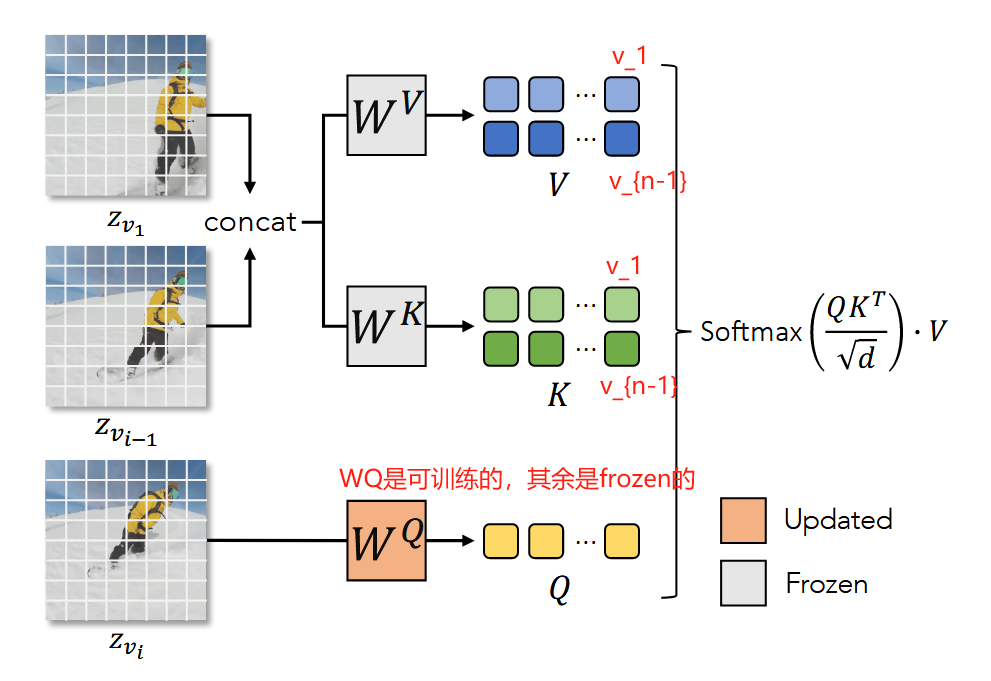
在ST-Attn模块的forward中,
K
,
V
K, V
K,V是这么计算的:
		# 表示上一帧的索引
		former_frame_index = torch.arange(video_length) - 1  # [-1, 0, 1, ..., n - 1]
        former_frame_index[0] = 0  # [0, 0, 1, ...]

		key = rearrange(key, "(b f) d c -> b f d c", f=video_length)  # 维度从(8, 256*256, 320) 到 (1, 8, 256*256, 320)
		# 将第一帧(f维索引为0)和上一帧(f维索引为idx - 1) 在sequence length维 concat起来
        key = torch.cat([key[:, [0] * video_length], key[:, former_frame_index]], dim=2)
        key = rearrange(key, "b f d c -> (b f) d c")  # (8, 2*256*256, 320)

		# value 同理
        value = rearrange(value, "(b f) d c -> b f d c", f=video_length)
        value = torch.cat([value[:, [0] * video_length], value[:, former_frame_index]], dim=2)
        value = rearrange(value, "b f d c -> (b f) d c")  # (8, 2*256*256, 320)

		# 因此QK^T 维度为 (8, 256*256, 2*256*256), Attn score的维度为(8, 256*256, 320)
2.4.2 DownBlock3D
DownBlock3D和CrossAttnDownBlock3D基本一致, 但其每一层只有ResNet block, 而没有Attention Block了. 不再赘述.
2.5 上采样
上采样的整体流程和降采样很相似, 无非是每次hidden states要首先与下采样部分对应block的输出结果concat, 熟悉UNet的同学应该不会陌生. 也就是forward的计算里多了这么几行:
		for resnet, attn in zip(self.resnets, self.attentions):
            # pop res hidden states
            res_hidden_states = res_hidden_states_tuple[-1]  # 每次取出downsample对应的hidden state
            res_hidden_states_tuple = res_hidden_states_tuple[:-1]
            hidden_states = torch.cat([hidden_states, res_hidden_states], dim=1)  # concat作为新的
上采样层同样用了前述的各种Attention.
3. 训练
在训练过程中, 我们激活特定的权重, 而将其他权重都冻住. 激活的权重就是本文提出的几个Attention中的映射矩阵:
	trainable_modules: Tuple[str] = (
        "attn1.to_q",
        "attn2.to_q",
        "attn_temp",
    ),

   for name, module in unet.named_modules():
        if name.endswith(tuple(trainable_modules)):
            for params in module.parameters():
                params.requires_grad = True
随后进行500轮的训练, 在每一轮中, 我们随机采样视频中的8帧, 以及对应的文本prompt, 按照标准的Diffusion模型训练流程即可:
- 用VAE的encoder提取视频帧特征, 用CLIP的text encoder提取文本特征
- 从标准高斯分布采样噪声 z z z
- 随机采样一个时间步 t t t
- 按照时间步 t t t加噪, 得到noisy latent z t z_t zt
- 用UNet预测初始噪声 z ~ \tilde{z} z~
- 计算Fisher散度, 即 z ~ \tilde{z} z~和 z z z的MSE loss.
- 反向传播. 更新优化器, lr scheduler
4. 推理
注意在使用diffusers库时, 推理过程最好继承DiffusionPipeline类, 在初始化函数也要把UNet, VAE, tokenizer这些都传进来. 遵循的流程也是:
- 用CLIP的text encoder提取文本特征
- 生成随机噪声
- 倒序时间步, 每一步用UNet预测从 t − 1 t-1 t−1到 t t t加的噪声, 并去噪
- 用VAE Decoder生成视频
一个细节: 在训练过程中, 在用VAE encoder提取视觉特征后, 将特征乘以了0.18215:
latents = vae.encode(pixel_values).latent_dist.sample()
latents = rearrange(latents, "(b f) c h w -> b c f h w", f=video_length)
latents = latents * 0.18215
当然, 在去噪过程从latent用VAE decoder生成视频时, 也需要反缩放回去:
	def decode_latents(self, latents):
        video_length = latents.shape[2]
        latents = 1 / 0.18215 * latents
        latents = rearrange(latents, "b c f h w -> (b f) c h w")
将 VAE encoder 提取的特征乘以 0.18215 主要是为了将特征空间中的数据缩放到适合 UNet 输入的尺度. VAE 编码器的输出是latent variables, 这些变量的范围通常在一个较大的范围内(通常是接近标准正态分布的范围). 为了让后续的 UNet 模型能够稳定地处理这些潜在变量, 需要对这些特征进行缩放.
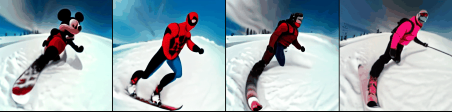
6. 运行结果
我们以一个人在滑雪的原始视频为例, 用如下的四个prompt:
    - "mickey mouse is skiing on the snow"
    - "spider man is skiing on the beach, cartoon style"
    - "wonder woman, wearing a cowboy hat, is skiing"
    - "a man, wearing pink clothes, is skiing at sunset"
在第100 peoch, 生成结果:
在第300 epoch, 生成结果:
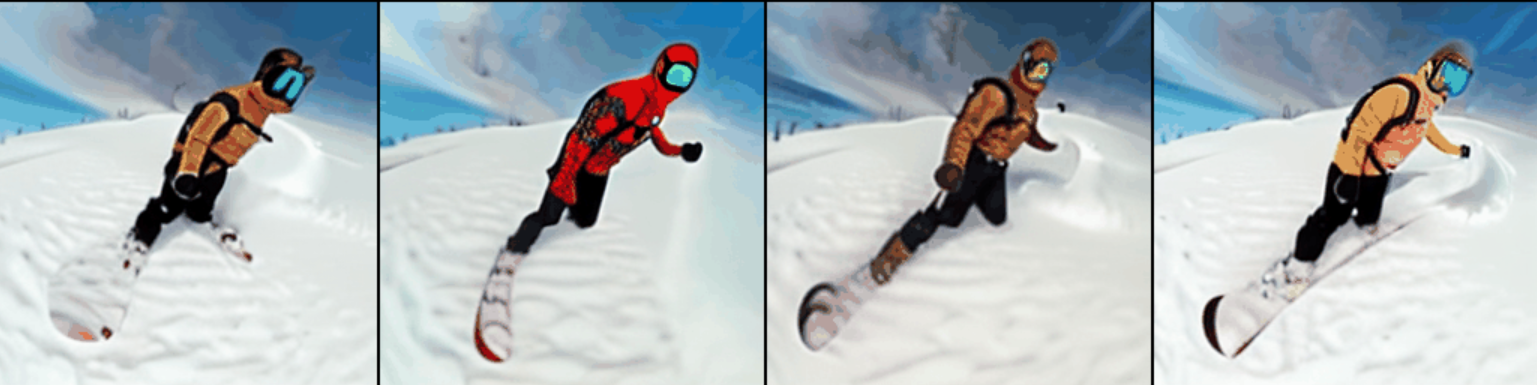
由此可以看出随着时间的增加, 反而偏向于失败. 我认为原因是, 在初期能够生成比较好的结果, 是因为SD有比较好的world knowledge, 而随着采样的增加, 我们训练的约束是原视频, 而不是SD在训练过程中的"目标图像" (因此这种方式的Video editing和SD的训练目标其实是不同的), 因此, 随着MSE loss的监督, 生成的视频只能和原视频越来越像.


 被折叠的 条评论
为什么被折叠?
被折叠的 条评论
为什么被折叠?
 到【灌水乐园】发言


