


function [Xi,Yi,Zi] = polarplot3d(Zp,varargin)
% POLARPLOT3D  Plot a 3D surface from polar coordinate data
%   [Xi,Yi,Zi] = polarplot3d(Zp,varargin)
%
% Input
%   Zp        A two dimensional matrix of input magnitudes or intensities.
%      Each column of Zp contains information along a single meridian. Each row
%      of Zp contains information at a single radius. The direction sense of the
%      rows and columns is determined by the relative order of the angular and
%      radial range vectors.  By default Zp is increasing in radius down each
%      column and increasing in angle along each row in the counter-clockwise
%      direction. The default plot is a full 360 degree surface plot with unit
%      radius.
%
%   varargin  'property',value pairs that modify plot characteristics.
%      Property names must be specified as quoted strings. Property names and
%      their values are not case sensitive. For each property the default value
%      is given below.  All properties are optional.  They may be given in any
%      order.
%
%   'PlotType'       'surfn'   surface plot,               no mesh (default)
%                    'surfcn'  surface plot with contours, no mesh
%                    'surfc'   surface plot with contours
%                    'surf'    surface plot
%                    'mesh'    mesh    plot
%                    'meshc'   mesh    plot with contours
%                    'contour' 2D contour plot
%                       Use 'ContourLines' to set the number of contours.
%                    'wire'    wireframe polar grid plot only, no surface plot
%                       A wireframe polar grid is plotted without a surface.
%                    'off'     no surface plot
%                       The data is interpolated to a new grid according to
%                       the 'MeshScale' property and transformed to Cartesian
%                       coordinates.
%
%   'AngularRange'   scalar or vector, radians (default = [0 2*pi])
%   'RadialRange'    scalar or vector          (default = [0 1])
%      If a scalar is given for either range it is used as the maximum value and
%      zero is used for the minimum.  If a two element vector is given, columns
%      (or rows) are evenly spaced between these values.  Otherwise the number
%      of elements must match the size of the corresponding dimension of Zp and
%      specifies the location of each column (or row).  If the vector values are
%      decreasing the corresponding dimension of Zp is reversed.
%
%   'ColorData'      Matrix of color values, size must be equal to size(Zp)
%      The default coloring is according to the magnitude of Zp.  For example
%      specifying gradient(Zp) colors the plot according to slope in the radial
%      direction.  Similarly gradient(Zp.').' colors the surface according to
%      slope in the azimuthal direction.
%
%   'CartOrigin'     Cartesian axis origin, 3 element vector (default = [0 0 0])
%      The center of the polar plot is translated to this location.
%
%   'MeshScale'      Mesh scale factors, 2 element vector (default = [1 1])
%      The data is interpolated to a new mesh size. Values > 1 increase mesh
%      element size and values < 1 decrease mesh element size.
%
%   'TickSpacing'    Spacing of polar tick marks in degrees (default = 10)
%      Every other tick mark is labeled. To supress tick marks specify zero,
%      an empty vector or an increment value greater than 180.
%
%   'PolarGrid'      Polar grid density (2 element cell array) (default = {10 8})
%      Number of grid sections in the radial and azimuthal directions.  A value
%      of 1 eliminates a grid direction from the plot. If a vector is specified
%      for a direction, gridlines are drawn at the specified locations.
%
%   'GridScale'      Smoothness of contoured grid lines (default = [40 40])
%      Larger values make the grid lines smoother.
%
%   'GridStyle'      Style of polar grid lines (default = ':' dotted line)
%      Plotting style for the radial and azimuthal grid lines.  Any format
%      supported by the plot function can be used: '-' solid, ':' dotted,
%      '-.' dashdot or '--' dashed.
%
%   'ContourLines'   Scalar (number of contours) or a vector (contour locations)
%      Either the number of contours or the location of contour lines is specified.
%      The default is auto selection by the contour function.
%
%   'AxisLocation'   'surf'    polar axis along edge of surface     (default)
%                    'min'     polar axis at minimum Zp for largest radius
%                    'max'     polar axis at maximum Zp for largest radius
%                    'mean'    polar axis at mean    Zp for largest radius
%                    'top'     polar axis at top     of plot box
%                    'bottom'  polar axis at bottom  of plot box
%                    value     polar axis is drawn at specified height
%                    'off'     no polar axis
%
%   'RadLabels'   Number of radial labels (default = 0)
%      The inner and outer most radii are not labeled. Labels are equally spaced
%      within the radial range of the data.
%
%   'RadLabelLocation'  Radial label location (2 element cell array) (default = {0 'max'})
%      The first elemenent is the azimuthal location of the radial labels in
%      degrees. The second element is the sagittal location of the labels. The
%      following values are allowed. If a value is given it can be a scalar or
%      a vector the same length as the value of the 'RadLabels' property.
%
%                    'surf'    above the surface at each theta,R
%                    'min'     at minimum value of Zp
%                    'max'     at maximum value of Zp (default)
%                    'mean'    at mean    value of Zp
%                    'top'     at the top    of the plot box
%                    'bottom'  at the bottom of the plot box
%                    value     at the specified height(s)
%                    'off'     no radial labels
%
%   'PolarDirection' 'ccw'     0 degs along +x axis, angles increase ccw (default)
%                    'cw'      0 degs along +y axis, angles increase cw
%                              This makes a compass-style polar grid.
%
%   'InterpMethod'   'cubic'   bicubic          interpolation on Zp (default)
%                    'linear'  bilinear         interpolation on Zp
%                    'spline'  spline           interpolation on Zp
%                    'nearest' nearest neighbor interpolation on Zp
%
%   'PolarAxisColor' color of the polar axis    (default = 'black')
%   'GridColor'      color of polar grid lines  (default = 'black')
%   'TickColor'      color of polar tick marks  (default = 'black')
%   'TickLabelColor' color of polar tick labels (default = 'black')
%   'RadLabelColor'  color of radial labels     (default = 'black')
%
%   Additional 'property',value pairs are applied to the current
%   axis using the set() command after the polar plot is drawn.
%
% Output
%   Xi,Yi,Zi   Cartesian locations corresponding to polar coordinates (T,R,Zp)
%              T and R are created from AngularRange and RadialRange arguments
%              using meshgrid and converted to Cartesian coordinates with
%              pol2cart.  Xi,Yi,Zi are square matrices with size equal to the
%              dimensions of Zp after interpolation.  Matrix sizes are reduced
%              or enlarged by the MeshScale property.
%
% Notes        Zp is the only required input argument
%              If no input arguments are given an example plot is produced
%              and this help text is displayed in the command window.
%
% ----
% Example
%    [t,r] = meshgrid(linspace(0,2*pi,361),linspace(-4,4,101));
%    [x,y] = pol2cart(t,r);
%    P = peaks(x,y);                       % peaks function on a polar grid
%
%                                          % draw 3d polar plot
%    figure('Color','white','NumberTitle','off','Name','PolarPlot3d v4.3');
%    polarplot3d(P,'PlotType','surfn','PolarGrid',{4 24},'TickSpacing',8,...
%                  'AngularRange',[30 270]*pi/180,'RadialRange',[.8 4],...
%                  'RadLabels',3,'RadLabelLocation',{180 'max'},'RadLabelColor','red');
%
%                                          % set plot attributes
%    set(gca,'DataAspectRatio',[1 1 10],'View',[-12,38],...
%            'Xlim',[-4.5 4.5],'Xtick',[-4 -2 0 2 4],...
%            'Ylim',[-4.5 4.5],'Ytick',[-4 -2 0 2 4]);
%    title('polarplot3d example');
%
% ----
% Versions
% 1    Original function based on POLAR3D by J De Freitas
% 2    Changed argument method to 'property',value pairs using PARSE_PV_PAIRS by J. D'Errico
% 2.1  Added 'ColorData' property
% 2.2  Updated contour plot implementation for meshc, surfc and surfcn plot types
% 2.3  Added radial and azimuthal mesh scale factors
% 2.4  Added 'CartOrigin' property
% 2.5  Added 'PolarAxisColor', 'GridColor', 'TickColor' and 'TickLabelColor' properties
% 2.6  Added 'PolarDirection' and 'GridScale' properties
% 3    Removed PARSE_PV_PAIRS dependency
% 4    Support for non-uniform grid spacing. Removed redundant 'MeshL' plot type
% 4.1  Replaced optional 'PlotProps' cell argument with 'property',value list
% 4.2  Added 'RadLabels', 'RadLabelLocation' and 'RadLabelColor' properties

% -- Help

% Polarplot3d was called without arguments
% Draw an example in a new figure and display help text
if nargin < 1
   [t,r] = meshgrid(linspace(0,2*pi,361),linspace(-4,4,101));
   [x,y] = pol2cart(t,r);
   P = peaks(x,y);                       % peaks function on a polar grid

                                         % draw 3d polar plot
   figure('Color','white','NumberTitle','off','Name','PolarPlot3d v4.3');
   polarplot3d(P,'PlotType','surfn','PolarGrid',{4 24},'TickSpacing',8,...
                 'AngularRange',[30 270]*pi/180,'RadialRange',[.8 4],...
                 'RadLabels',3,'RadLabelLocation',{180 'max'},'RadLabelColor','red');

                                         % set plot attributes
   set(gca,'DataAspectRatio',[1 1 10],'View',[-12,38],...
           'Xlim',[-4.5 4.5],'Xtick',[-4 -2 0 2 4],...
           'Ylim',[-4.5 4.5],'Ytick',[-4 -2 0 2 4]);
   title('polarplot3d example');
                                         % display help text
   error(['No input arguments given\n'...
          'Please consult the help text and the example plot\n'...
          '--------\n%s'],help(mfilename));
end


%-- Parse and validate input arguments

% Allowed argument string for property values
plst = {'mesh','meshc','wire',...
        'surf','surfc','surfn','surfcn','contour','off'};
alst = {'off','const','min','max','mean','surf','top','bottom'};
rlst = {'off','const','min','max','mean','surf','top','bottom'};
mlst = {'cubic','linear','spline','nearest'};
dlst = {'ccw','cw'};
glst = {'-',':','-.','--'};

% Set up property structure with default values
p.angularrange      = [0 2*pi];   % angular range
p.radialrange       = [0 1];      % radial  range
p.plottype          = 'surfn';    % surface plot, no rectangular grid
p.meshscale         = [1 1];      % no mesh scaling
p.polargrid         = {10 8};     % number of radial and azimuthal sections
p.gridscale         = [40 40];    % 40x scaling for smooth grid interpolation
p.cartorigin        = [0 0 0];    % Cartesian origin
p.tickspacing       = 10;         % ten degree tick mark spacing
p.radlabels         =  0;         % number of radial grid labels
p.axislocation      = '';         % polar axis location
p.radlabellocation  = '';         % radial label location
p.polardirection    = 'ccw';      % default polar axis direction
p.interpmethod      = 'cubic';    % bicubic interpolation
p.colordata         = [];         % default coloring according to Zp values
p.contourlines      = '';         % default contour specification
p.gridcolor         = 'black';    % default overlay grid line color
p.gridstyle         = '';         % style of grid lines: '-' ':' '-.' '--'
p.polaraxiscolor    = 'black';    % default polar axis color
p.tickcolor         = 'black';    % default polar tick color
p.ticklabelcolor    = 'black';    % default polar tick label color
p.radlabelcolor     = 'black';    % default radial label color
p.plotprops         = {};         % no additional plot properties

% Parse property value pairs, replace defaults with values specified by caller
try
   [p,leftovers] = structrecon(pv2struct(varargin{:}),p);
   p.plotprops   = struct2pv(leftovers);
catch ERR
   error('Error parsing varargin list\n??? %s',ERR.message);
end

% Check input data size
[Zrows,Zcols] = size(Zp);
if (Zrows < 5) || (Zcols < 5)
   error('Input matrix size must be greater than 4 x 4');
end

% Check plot type specification
if ~ischar(p.plottype) || isempty(matchstr2lst(lower(p.plottype),plst))
   error('Invalid ''PlotType'' property value');
end
p.plottype = lower(p.plottype);

% Choose default polar axis location
if isequal(p.axislocation,'')
   if ~isempty(matchstr2lst(p.plottype,{'meshc','surfc','surfcn'}))
        p.axislocation = 'bottom';       % plot box bottom for contour plots
   else p.axislocation = 'surf';         % along perimeter of surface otherwise
   end
end

% User specified polar axis location as a numeric value
if isnumeric(p.axislocation)
   [r,c] = size(p.axislocation);
   if (((r ~= 1) || (c ~= 1)) || ~isnumeric(p.axislocation))
      error('''AxisLocation'' property value must be scalar, positive and real');
   end
   polax          = p.axislocation;
   p.axislocation = 'const';
end

% Check polar axis location specification
if ~ischar(p.axislocation) || isempty(matchstr2lst(lower(p.axislocation),alst))
   error('Invalid ''AxisLocation'' property value');
end
p.axislocation = lower(p.axislocation);

% Check polar axis direction specification
if ~ischar(p.polardirection) || isempty(matchstr2lst(lower(p.polardirection),dlst))
   error('Invalid ''PolarDirection'' property value');
end
p.polardirection = lower(p.polardirection);

% Check grid scaling specification
p.gridscale = p.gridscale(:)';
if ~isnumeric(p.gridscale) || any(p.gridscale <= 0)
   error('Non-numeric or non-positive grid scale parameter');
end
if length(p.gridscale) ~= 2
   error('''GridScale'' property must be a two element numeric vector');
end

% Check angular range vector
p.angularrange = p.angularrange(:);
if ~isnumeric(p.angularrange)
   error('''AngularRange'' property value must be numeric');
end
if isscalar(p.angularrange), p.angularrange = [0; p.angularrange]; end
if length(p.angularrange) == 2
   p.angularrange = linspace(p.angularrange(1),p.angularrange(2),Zcols).';
end
if ~ismono(p.angularrange)
   error('''AngularRange'' vector must be monotonic');
end
if length(p.angularrange) ~= Zcols
   error('''AngularRange'' size must match number of columns in input matrix');
end

% Check radial range vector
p.radialrange = p.radialrange(:);
if ~isnumeric(p.radialrange)
   error('''RadialRange'' property value must be numeric');
end
if isscalar(p.radialrange), p.radialrange = [0; p.radialrange]; end
if length(p.radialrange) == 2
   p.radialrange = linspace(p.radialrange(1),p.radialrange(2),Zrows).';
end
if ~ismono(p.radialrange)
   error('''RadialRange'' vector must be monotonic');
end
if length(p.radialrange) ~= Zrows
   error('''RadialRange'' size must match number of rows in input matrix');
end

% Angular and radial range vectors define data order
[Tmin,Tmax] = deal(min(p.angularrange),max(p.angularrange));   % Tmin < Tmax
[Rmin,Rmax] = deal(min(p.radialrange ),max(p.radialrange ));   % Rmin < Rmax

% Reflect Zp left-right and/or up-down depending on angular and radial ranges
if p.angularrange(1) > p.angularrange(end), Zp = fliplr(Zp); end
if p.radialrange (1) > p.radialrange (end), Zp = flipud(Zp); end

% Angular range cannot be more than one full circumference
if abs(Tmax - Tmin) > 2*pi
   error('Angular range cannot be greater than 2*pi');
end

% Check radial and azimuthal polar grid density
p.polargrid = p.polargrid(:);
if length(p.polargrid) ~= 2 || ~iscell(p.polargrid)
   error('''PolarGrid'' property value must be a two element numeric cell array');
end
[radgrid,azmgrid] = deal(p.polargrid{1},p.polargrid{2});

% Check azimuthal grid density
if ~isnumeric(azmgrid)
   error('Non-numeric azimuthal grid parameter');
end
if isempty(azmgrid) || (length(azmgrid)==1 && azmgrid == 0)
   azmgrid = 1;
end
if length(azmgrid) == 1
   azmgrid = linspace(Tmin,Tmax,azmgrid+1).';
end

% Check radial grid density
if ~isnumeric(radgrid)
   error('Non-numeric radial grid parameter');
end
if isempty(radgrid) || (length(radgrid)==1 && radgrid==0)
   radgrid = 1;
end
if length(radgrid) == 1
   radgrid = linspace(Rmin,Rmax,radgrid+1).';
end

% Check number of radial grid labels
if ~isnumeric(p.radlabels)
   error('''RadialLablels'' property value must be numeric');
end

% Check radial label location, {azimuthal, sagittal}
if isempty(p.radlabellocation)
   p.radlabellocation = {0 'surf'};
end
if ~iscell(p.radlabellocation) || numel(p.radlabellocation) ~= 2
   error('''RadLabelLocation'' property must be a 2 element cell array');
end
azimuth_radax = p.radlabellocation{1};
if ~isnumeric(azimuth_radax) || azimuth_radax < 0 || azimuth_radax > 360
   error('azimuthal radial location must be between 0 and 360 degrees');
end
p.radlabellocation = p.radlabellocation{2};
if isnumeric(p.radlabellocation)
   sagittal_radax     = p.radlabellocation;
   p.radlabellocation = 'const';
end
if ~ischar(p.radlabellocation) || isempty(matchstr2lst(lower(p.radlabellocation),rlst))
   error('Invalid ''RadLabelLocation'' property value');
end
p.radlabellocation = lower(p.radlabellocation);

% Check mesh scale factor property value
if isscalar(p.meshscale), p.meshscale = [p.meshscale p.meshscale]; end
if ~isnumeric(p.meshscale) || any(p.meshscale <= 0)
   error('''MeshScale'' property values must be positive and real');
end

% Check tick spacing property value
if ~isempty(p.tickspacing) && (~isscalar(p.tickspacing) || ~isnumeric(p.tickspacing))
   error('''TickSpacing'' property value must be a scalar numeric value or empty');
end

% Check contour lines property value
if ~isnumeric(p.contourlines) && ~isequal(p.contourlines,'')
   error('''ContourLines'' property value must be numeric');
end
p.contourlines = p.contourlines(:);

% Check grid line style property value, default depends on plottype
if isempty(p.gridstyle)
   if isequal(p.plottype,'contour'), p.gridstyle = ':';    % dotted line
   else                              p.gridstyle = '-';    % solid  line
   end
end
if ~ischar(p.gridstyle) || isempty(matchstr2lst(lower(p.gridstyle),glst))
   error('Invalid ''GridStyle'' property value');
end

% Check interpolation method
p.interpmethod = lower(p.interpmethod);
if ~ischar(p.interpmethod) || isempty(matchstr2lst(p.interpmethod,mlst))
   error('Invalid ''InterpMethod'' property value');
end

% Check if mesh scale factor is compatible with input data dimension
if round(min([Zrows Zcols]./p.meshscale)) < 4
   error('Mesh scale factor is too large, not enough data remaining to plot');
end

% Choose default color matrix
if isempty(p.colordata), p.colordata = Zp; end       % surface height coloring

% Check color matrix
if ~isnumeric(p.colordata) || ~isequal(size(p.colordata),[Zrows,Zcols])
   error('Color matrix must be numeric and the same size as Zp');
end

% Polar axis z location is a constant for contour plots
if isequal(p.plottype,'contour') && ~isequal(p.axislocation,'off')
   polax = 0;
   p.axislocation = 'const';
end

% Check Cartesian origin
if isempty(p.cartorigin) || ~isnumeric(p.cartorigin)
   error('Cartesian origin must be numeric');
end
if length(p.cartorigin)<3, p.cartorigin(3) = 0; end


%-- Create polar grid and interpolate data

% Create radius and angle vectors and polar grid for input data matrix
rho  = p.radialrange;                                % radius vector
angl = p.angularrange;                               % angle  vector
[xx,yy] = meshgrid(angl,rho);                        % mesh   matrices
Zi = Zp;                                             % z's == input data
Ci = p.colordata;                                    % colormap

% No interpolation for uniform scaling
if isequal(p.meshscale,[1 1])                        % uniform scaling
   Xi = rho * cos(angl.');                           % matrix of x's
   Yi = rho * sin(angl.');                           % matrix of y's

% Create a new grid and interpolation data
else
   q    = fix([Zrows Zcols]./p.meshscale);           % new mesh size
   rho  = linspace(Rmin,Rmax,q(1));                  %     radius vector
   angl = linspace(Tmin,Tmax,q(2));                  %     angle  vector
   [theta,rad] = meshgrid(angl,rho);                 % create polar grid
   T  = interp2(xx,yy,Zp,theta,rad,p.interpmethod);  % interpolate Zp to grid
   Ci = interp2(xx,yy,Ci,theta,rad,p.interpmethod);  % interpolate color
   [Xi,Yi,Zi] = pol2cart(theta,rad,T);               % convert to Cartesian
end

% Swap x,y for clockwise polar plot
if isequal(p.polardirection,'cw')
   [Xi,Yi] = deal(Yi,Xi);
end

% Offset grid data to Cartesian origin
Xi = Xi + p.cartorigin(1);
Yi = Yi + p.cartorigin(2);
Zi = Zi + p.cartorigin(3);


%-- Plot the surface

switch p.plottype
   case 'wire',    grid on;
   case 'meshc',   mesh(Xi,Yi,Zi,Ci);
                   addcontours(Xi,Yi,Zi,p.contourlines);
   case 'mesh',    mesh (Xi,Yi,Zi,Ci);
   case 'surf',    surf (Xi,Yi,Zi,Ci);
   case 'surfc',   surf (Xi,Yi,Zi,Ci);
                   addcontours(Xi,Yi,Zi,p.contourlines);
   case 'surfn',   surf (Xi,Yi,Zi,Ci,'LineStyle','none');
   case 'surfcn',  surf (Xi,Yi,Zi,Ci,'LineStyle','none');
                   addcontours(Xi,Yi,Zi,p.contourlines);
   case 'contour', contour(Xi,Yi,Zi,p.contourlines);
                   axis equal; xlim(xlim*1.1); ylim(ylim*1.1);
                   set(gca,'visible','off');
                   set(get(gca,'xlabel'),'visible','on');
                   set(get(gca,'ylabel'),'visible','on');
                   set(get(gca,'title'), 'visible','on');
end


%-- Plot the polar axis

% Axis and tick label attributes
fontargs = {'FontName','Arial','FontSize',10,'FontWeight','bold'};

if ~isequal(p.axislocation,'off')

   % Create polar axis data just outside the largest radius
   xa = Rmax * 1.005 .* cos(angl) + p.cartorigin(1);
   ya = Rmax * 1.005 .* sin(angl) + p.cartorigin(2);

   % Set polax to z location of polar axis
   switch p.axislocation
      case 'min',    polax = min (Zi(end,:));
      case 'max',    polax = max (Zi(end,:));
      case 'mean',   polax = mean(Zi(end,:));
      case 'top',    zlim  = get(gca,'zlim'); polax = zlim(2);
      case 'bottom', zlim  = get(gca,'zlim'); polax = zlim(1);
   end

   % Z values for polar axis
   if isequal(p.axislocation,'surf')
        za = Zi(end,:);                      % vary along edge of surface
   else za = zeros(size(xa)) + polax;        % constant location
   end

   % Swap x,y for clockwise polar plot
   if isequal(p.polardirection,'cw'), [xa,ya] = deal(ya,xa); end

   % Plot the polar axis
   hold on;
   line(xa,ya,za,'Color',p.polaraxiscolor,'LineWidth',1);

   % Add tick marks and labels
   if ~isempty(p.tickspacing) && p.tickspacing > 0 && p.tickspacing <= 180

      % Create polar axis tic marks at p.tickspacing intervals
      ts = 180/p.tickspacing;
      ta = pi/ts * (round(Tmin*ts/pi):1:round(Tmax*ts/pi));
      tr = Rmax  * [1.005; 1.03; 1.1];
      xt = tr * cos(ta) + p.cartorigin(1);
      yt = tr * sin(ta) + p.cartorigin(2);

      % Z values for polar tick marks
      if isequal(p.axislocation,'surf')
           zt = interp1(angl,za,ta,'linear');    % vary along edge of surface
      else zt = zeros(1,length(ta)) + polax;     % constant location
      end

      % Label every other tick mark
      nl = round(length(ta)/2);

      % Beginning and end of a full polar axis are identical, label once
      if abs(Tmin-Tmax) == 2*pi, nl = nl-1; end

      % Swap x,y for clockwise polar plot
      if isequal(p.polardirection,'cw'), [xt,yt] = deal(yt,xt); end

      % Draw the tick marks
      line(xt(1:2,:),yt(1:2,:),[zt; zt],'Color',p.tickcolor);

      % Add tick labels
      for k = 2 * (1:nl) - 1
         text(xt(3,k),yt(3,k),zt(k),num2str(ta(k)*180/pi),...
              'HorizontalAlignment','Center',fontargs{:},'Color',p.ticklabelcolor);
      end
   end
   hold off;
end


% -- Add radial labels

if p.radlabels > 0 && ~isequal(p.radlabellocation,'off')

   % Find x,y locations of radial labels
   ta = azimuth_radax*pi/180;
   tr = linspace(Rmin,Rmax,p.radlabels+2);
   tr(1) = []; tr(end) = [];                     % delete inner,outer labels
   xt = tr * cos(ta) + p.cartorigin(1);
   yt = tr * sin(ta) + p.cartorigin(2);

   % Swap x,y for clockwise polar plot
   if isequal(p.polardirection,'cw'), [xt,yt] = deal(yt,xt); end

   % Set sagittal_radax to z location of radial labels
   switch p.radlabellocation
      case 'min',    sagittal_radax = min (Zi(:));
      case 'max',    sagittal_radax = max (Zi(:));
      case 'mean',   sagittal_radax = mean(Zi(:));
      case 'top',    zlim = get(gca,'zlim'); sagittal_radax = zlim(2);
      case 'bottom', zlim = get(gca,'zlim'); sagittal_radax = zlim(1);
   end

   % Z values for radial labels
   if isequal(p.radlabellocation,'surf')
        zt = interp2(xx,yy,Zp,ta,tr,p.interpmethod);   % vary with surface
   else
      sagittal_radax(length(tr)+1:end) = [];
      sagittal_radax(end+1:length(tr)) = sagittal_radax(end);
      zt = zeros(1,length(tr)) + sagittal_radax;     % constant location
   end

   % Add radial labels to the plot
   hold on;
   for k = 1:length(tr)
      text(xt(k),yt(k),zt(k),num2str(tr(k)),...
         'HorizontalAlignment','Center',fontargs{:},'Color',p.radlabelcolor);
   end
   hold off;
end


%-- Draw polar grid lines

r = length(radgrid);
m = length(azmgrid);

% Is there more than one radial or azimuthal section?
if r > 1 || m > 1

   % Allocate space for grid lines
   u    = p.gridscale(1);
   v    = p.gridscale(2);
   rho  = zeros(1,(r-1)*u+1);
   angl = zeros(1,(m-1)*v+1);

   % Fill in grid vectors between points so the interpolated grid follows
   % surface contours smoothly and the azimuthal grid lines are circular.
   for k = 1:r-1
      rho((k-1)*u+1:(k*u)+1) = linspace(radgrid(k),radgrid(k+1),u+1);
   end
   for k = 1:m-1
      angl((k-1)*v+1:(k*v)+1) = linspace(azmgrid(k),azmgrid(k+1),v+1);
   end

   % Interpolate data to a fine mesh to produce smooth grid lines
   [theta,rad] = meshgrid(angl,rho);                 % create polar grid
   T = interp2(xx,yy,Zp,theta,rad,p.interpmethod);   % interpolate to grid
   [xi,yi,zi] = pol2cart(theta,rad,T);               % convert to Cartesian
   xi = xi + p.cartorigin(1);                        % translate center, x
   yi = yi + p.cartorigin(2);                        %                   y
   zi = zi + p.cartorigin(3);                        %                   z

   % Swap x,y for clockwise polar plot
   if isequal(p.polardirection,'cw')
      [xi,yi] = deal(yi,xi);
   end

   % In-plane grid lines for contour plots
   if isequal(p.plottype,'contour'), zi = zeros(size(zi)); end

   % draw radial grid lines in azimuthal direction (meridians)
   hold on;
   if length(azmgrid) > 2
      xr = xi(:,1:u:end);
      yr = yi(:,1:u:end);
      zr = zi(:,1:u:end);
      plot3(xr,yr,zr,p.gridstyle,'Color',p.gridcolor,'LineWidth',1);
   end

   % Draw azimuthal grid lines in radial direction (concentric arcs)
   if length(radgrid) > 2
      xm = xi(1:v:end,:);
      ym = yi(1:v:end,:);
      zm = zi(1:v:end,:);
      plot3(xm',ym',zm',p.gridstyle,'Color',p.gridcolor,'LineWidth',1);
   end
   hold off;
end

%-- Set axis font
if ~isequal(p.plottype,'off'), set(gca,fontargs{:}); end

%-- Apply additional properties to the plot
if ~isempty(p.plotprops), set(gca,p.plotprops{:}); end
end


%-- Local functions

% Add a contour plot to the current surface or mesh plot
function addcontours(x,y,z,levels)

if isempty(levels), levels = 16; end
hold on;
a    = get(gca,'zlim');
zpos = a(1);               % find smallest z value in 3d plot

% Add contours
[~,hh] = contour3(x,y,z,levels);

% Change all contour group positions to bottom of plot
for j = 1:length(hh)
   zz = get(hh(j),'Zdata');
   set(hh(j),'Zdata',zpos*ones(size(zz)));
end
end

% Structure reconciliation with a template
function [T,S] = structrecon(S,D)

% Check arguments, must have two structures
if ~(isstruct(S) && isstruct(D))
   error('input arguments must be structures');
end

T     = D;             % copy the template
fname = fields(T);     % make a list of field names

% Loop over all fields in the template, copy matching values from S
for k = 1:length(fname)
   % Process matching field names in S
   if isfield(S,fname{k})
      % Is this a substructure ?
      if isstruct(T.(fname{k})) && isstruct(S.(fname{k}))
         % Recursively process the substructure
         T.(fname{k}) = structrecon(S.(fname{k}),T.(fname{k}));
      % Not a substructure, copy field value from S
      else T.(fname{k}) = S.(fname{k});
      end
      S = rmfield(S,fname{k});
   end
end
end

% Convert an argument pairs cell array to a structure
function S = pv2struct(varargin)

% No inputs, return empty structure
if isempty(varargin), S = struct(); return; end

% Need pairs of inputs
if mod(length(varargin),2)==1
   error('number of arguments must be even');
end

% Odd elements of varargin are fields, even ones are values
% Store all field names in lower case
for k = 1:2:length(varargin)
   S.(lower(varargin{k})) = varargin{k+1};
end
end

% Convert a structure to an argument pairs cell array
function P = struct2pv(S)

% Check input argument
if ~isstruct(S), P = {}; return; end

% Get field names
n = fieldnames(S);

% Convert structure values to cell array
v = struct2cell(S);

% Combine names and values, return a 1xN cell array
P = {n{:}; v{:}};
P = P(:).';
end

% Match a string with a list of strings
function idx = matchstr2lst(str,strarray,opt)

if nargin < 2, return; end
idx = find(strncmpi(str,strarray,length(str))==1);
idx = idx(:);

if nargin > 2
   if     strcmpi(opt,'first'), idx = idx(1);
   elseif strcmpi(opt,'last'),  idx = idx(end);
   end
end
end

% Test monotonicity of a vector
function m = ismono(v)

[r,c] = size(v);       % size of input
if r == 1,             % row vector
   v = v';             %   transpose
   r = c; c = 1;       %   size
end

sgn   = sum(sign(diff(v,1,1)),1);  % sgn is r+1 or -(r+1) for monotonic columns
up    = sgn - repmat(r,1,c);       % subtract r to detect increasing (-1)
down  = sgn + repmat(r,1,c);       % add      r to detect decreasing (+1)
up  (up   < -1) = 0;               % force non-monotonic entries to zero
down(down >  1) = 0;

m = -(up + down);                  % flip sense of output so +1 is increasing

end
%% Examples of the polarplot3d function
% The peaks function on a polar grid
[t,r] = meshgrid(linspace(0,2*pi,361),linspace(-4,4,101));
[x,y] = pol2cart(t,r);
P = peaks(x,y);
% Define some angular and radial range vectors for example plots
t1 = 2*pi;
t2 = [30 270]*pi/180;
r1 = 4;
r2 = [.8 4];
t3 = fliplr(t2);
r3 = fliplr(r2);
t4 = [30 35 45 60 90 135 200 270]*pi/180;
r4 = [0.8:0.4:2.8 3:0.2:4];
% Axis property cell array
axprop = {'DataAspectRatio',[1 1 8],'View', [-12 38],...
'Xlim', [-4.5 4.5], 'Ylim', [-4.5 4.5],...
'XTick',[-4 -2 0 2 4], 'YTick',[-4 -2 0 2 4]};
%% Plot using default arguments
figure('color','white');
polarplot3d(P);
view([-18 76]);
%% Plot of an incomplete polar annulus, color is azimuthal gradient
figure('color','white');
polarplot3d(P,'plottype','surf','angularrange',t2,'radialrange',r2,...
'polargrid',{1 16},'tickspacing',8,'colordata',gradient(P),...
'plotprops',{'Linestyle','none'});
set(gca,axprop{:});
%% Surface plot with contours
figure('color','white');
polarplot3d(P,'plottype','surfcn','angularrange',t2,'radialrange',r2,...
'polargrid',{10 24},'tickspacing',15);
set(gca,axprop{:});
%% Surface plot with unequally spaced polar grid lines
figure('color','white');
polarplot3d(P,'plottype','surfn','radialrange',[min(r4) max(r4)],...
'angularrange',[min(t4) max(t4)],'polargrid',{r4 t4},'tickspacing',15);
set(gca,axprop{:});
%% Surface plot, compass convention, color is radial direction gradient
figure('color','white');
polarplot3d(P,'plottype','surfn','angularrange',t2,...
'radialrange',r2,'tickspacing',15,...
'polardirection','cw','colordata',gradient(P.').');
set(gca,axprop{:});
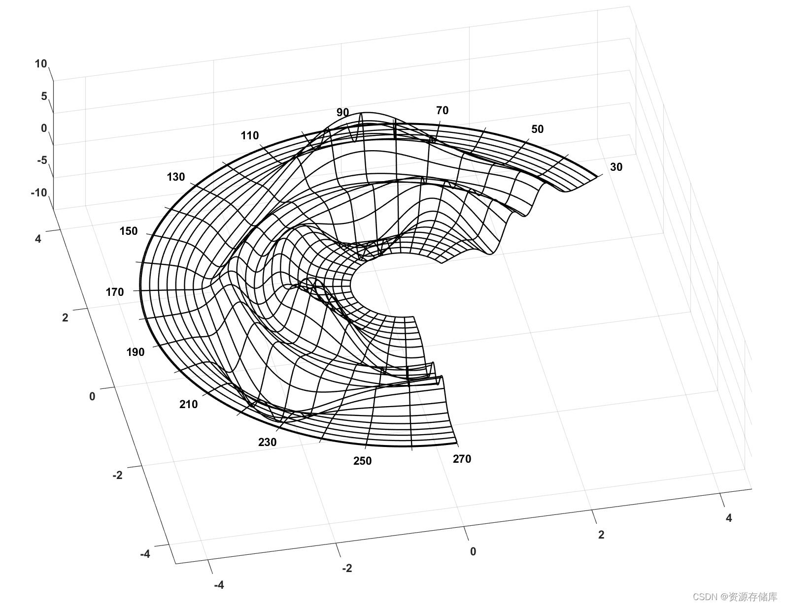
%% Mesh plot with polar axis at mean value, reversed angular sense
figure('color','white');
polarplot3d(P,'plottype','mesh','angularrange',t3,'radialrange',r2,...
'meshscale',2,'polargrid',{1 1},'axislocation','mean');
set(gca,axprop{:});
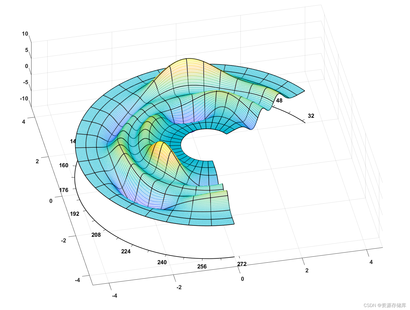
%% Mesh plot with polar axis along edge of surface
figure('color','white');
polarplot3d(P,'plottype','mesh','angularrange',t2,'radialrange',r2,...
'polargrid',{10 24},'tickspacing',8,...
'plotprops',{'Linestyle','none'});
set(gca,axprop{:});
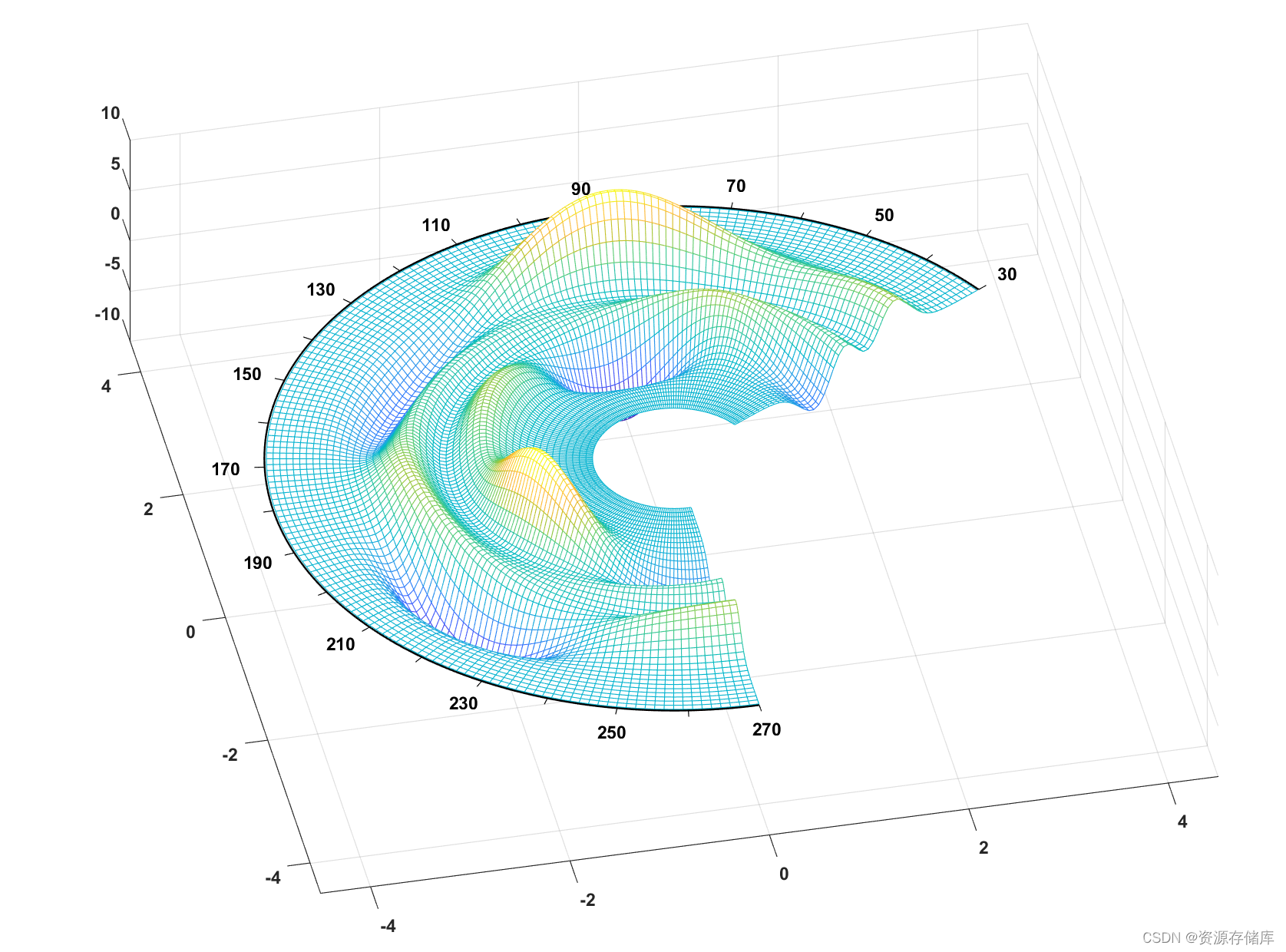
%% Mesh plot with contours, overlay 8 by 8 polar grid
figure('color','white');
polarplot3d(P,'plottype','meshc','angularrange',t2,'radialrange',r3,...
'meshscale',2,'polargrid',{8 8});
set(gca,axprop{:});
%% Wireframe plot
figure('color','white');
polarplot3d(P,'plottype','wire','angularrange',t2,'radialrange',r2,...
'polargrid',{24 24});
set(gca,axprop{:});
%% Surface and contour plot, reversed radial sense
cl = round(min(P(:))-1):0.4:round(max(P(:))+1);
figure('color','white');
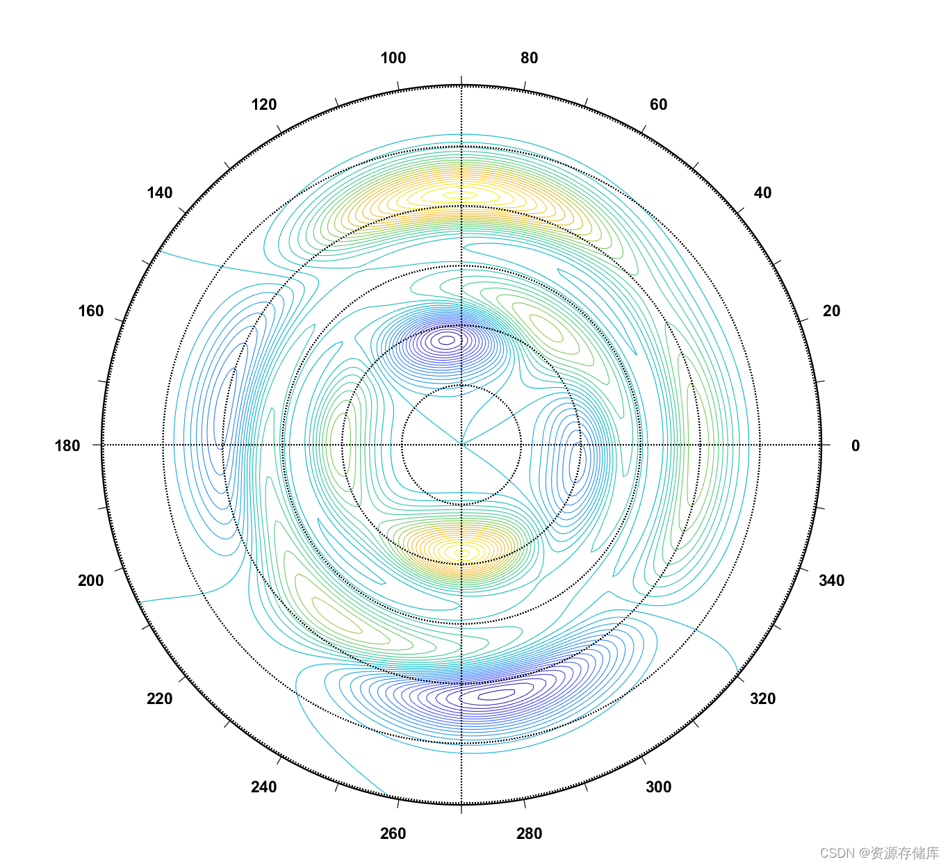
polarplot3d(P,'plottype','contour','polargrid',{6 4},'contourlines',cl);
set(gca,'dataaspectratio',[1 1 1],'view',[0 90]);


 7601
7601

 被折叠的 条评论
为什么被折叠?
被折叠的 条评论
为什么被折叠?
 到【灌水乐园】发言


