


 该博客展示了如何使用Python和matplotlib库来可视化三维人体姿态预测结果。代码首先定义了人体关节的名称及其在3D空间中的连接关系,然后定义了两个函数分别用于绘制2D和3D骨架。通过加载预训练模型的预测数据和真实数据,对比显示了预测的2D和3D姿势以及真实姿势。最后,通过一个示例展示了一组人物不同姿态的对比,包括2D、预测的3D和真实的3D姿态。
根据模型预测关节位置和真实关节位置画3维图
import pickle
import tensorflow as tf

import matplotlib
matplotlib.use('TkAgg')
import matplotlib.pyplot as plt
import numpy as np
from mpl_toolkits.mplot3d import Axes3D
import matplotlib.gridspec as gridspec


# Joints in H3.6M -- data has 32 joints, but only 17 that move; these are the indices.
H36M_NAMES = ['']*17
H36M_NAMES[0]  = 'LFoot'
H36M_NAMES[1]  = 'LKnee'
H36M_NAMES[2]  = 'LHip'
H36M_NAMES[3]  = 'RHip'
H36M_NAMES[4]  = 'RKnee'
H36M_NAMES[5]  = 'RFoot'
H36M_NAMES[6]  = 'Hip'
H36M_NAMES[7] = 'Belly'
H36M_NAMES[8] = 'Neck'
H36M_NAMES[9] = 'Head'
H36M_NAMES[10] = 'LHand'
H36M_NAMES[11] = 'LElbow'
H36M_NAMES[12] = 'LShoulder'
H36M_NAMES[13] = 'RShoulder'
H36M_NAMES[14] = 'RElbow'
H36M_NAMES[15] = 'RHand'
H36M_NAMES[16] = 'Nose'


def show3Dpose(channels, ax, lcolor="#3498db", rcolor="#e74c3c", add_labels=False): # blue, orange
  """
  Visualize a 3d skeleton

  Args
    channels: 96x1 vector. The pose to plot.
    ax: matplotlib 3d axis to draw on
    lcolor: color for left part of the body
    rcolor: color for right part of the body
    add_labels: whether to add coordinate labels
  Returns
    Nothing. Draws on ax.
  """

  assert channels.size == len(H36M_NAMES)*3, "channels should have 51 entries, it has %d instead" % channels.size
  vals = np.reshape( channels, (len(H36M_NAMES), -1) )

  I   = np.array([0, 1, 2, 3, 4, 3, 6, 7, 8,  9,  8,  11, 8,  13, 14, 10]) # start points
  J   = np.array([1, 2, 6, 4, 5, 6, 7, 8, 16, 16, 12, 12, 13, 14, 15, 11]) # end points
  LR  = np.array([0, 0, 0, 1, 1, 1, 0, 0, 0,  0,  0,  0,  1,  1,  1,  0], dtype=bool)#右半边的颜色

  # Make connection matrix
  for i in np.arange( len(I) ):
    x, y, z = [np.array( [vals[I[i], j], vals[J[i], j]] ) for j in range(3)]
    ax.plot(x, y, z, lw=2, c=lcolor if LR[i] else rcolor)#lw线条宽度
  #画点
  # lcolor = "#FF9500"
  # for i in np.arange(len(I)):
  #   x, y, z = vals[i]
  #   print(x,y,z)
  #   ax.scatter(x, y, z, lw=2, c=lcolor)#lw线条宽度

  RADIUS = 750 # space around the subject
  xroot, yroot, zroot = vals[6,0], vals[6,1], vals[6,2] #hip的位置
  ax.set_xlim3d([-RADIUS+xroot, RADIUS+xroot])
  ax.set_zlim3d([-RADIUS+zroot, RADIUS+zroot])
  ax.set_ylim3d([-RADIUS+yroot, RADIUS+yroot])
  ax.grid(True)

  if add_labels:
    ax.set_xlabel("x")
    ax.set_ylabel("y")
    ax.set_zlabel("z")

  # Get rid of the ticks and tick labels
  ax.set_xticks([])
  ax.set_yticks([])
  ax.set_zticks([])

  ax.get_xaxis().set_ticklabels([])
  ax.get_yaxis().set_ticklabels([])
  ax.set_zticklabels([])

  # Get rid of the panes (actually, make them white)
  white = (1.0, 1.0, 1.0, 0.0)

  # ax.w_xaxis.set_pane_color(white)
  # ax.w_yaxis.set_pane_color(white)
  # # Keep z pane
  #
  # Get rid of the lines in 3d
  ax.w_xaxis.line.set_color(white)
  ax.w_yaxis.line.set_color(white)
  ax.w_zaxis.line.set_color(white)


def show2Dpose(channels, ax, lcolor="#3498db", rcolor="#e74c3c", add_labels=False):
  """Visualize a 2d skeleton

  Args
    channels: 64x1 vector. The pose to plot.
    ax: matplotlib axis to draw on
    lcolor: color for left part of the body
    rcolor: color for right part of the body
    add_labels: whether to add coordinate labels
  Returns
    Nothing. Draws on ax.
  """


  assert channels.size == len(H36M_NAMES)*2, "channels should have 64 entries, it has %d instead" % channels.size
  vals = np.reshape(channels, (len(H36M_NAMES), -1) )

  I = np.array([0, 1, 2, 3, 4, 3, 6, 7, 8, 9, 8, 11, 8, 13, 14, 10])  # start points
  J = np.array([1, 2, 6, 4, 5, 6, 7, 8, 16, 16, 12, 12, 13, 14, 15, 11])  # end points
  LR  = np.array([0, 0, 0, 1, 1, 1, 0, 0, 0,  0,  0,  0,  1,  1,  1,  0], dtype=bool)#右半边的颜色

  # Make connection matrix
  for i in np.arange( len(I) ):
    x, y = [np.array( [vals[I[i], j], vals[J[i], j]] ) for j in range(2)]
    ax.plot(x, y, lw=2, c=lcolor if LR[i] else rcolor)

  # Get rid of the ticks
  ax.set_xticks([])
  ax.set_yticks([])

  # Get rid of tick labels
  ax.get_xaxis().set_ticklabels([])
  ax.get_yaxis().set_ticklabels([])

  RADIUS = 1000 # space around the subject
  xroot, yroot = vals[6,0], vals[6,1]
  ax.set_xlim([-RADIUS+xroot, RADIUS+xroot])
  ax.set_ylim([-RADIUS+yroot, RADIUS+yroot])
  if add_labels:
    ax.set_xlabel("x")
    ax.set_ylabel("z")

  ax.set_aspect('equal')


def get_data():
  path = 'results.pkl'

  f = open(path, 'rb')

  data = pickle.load(f)

  # f1 = open(r'F:/Python codes/pose_lcn/dataset/h36m_test.pkl', 'rb')
  # dataitem_gt = pickle.load(f1)
  return data


def get_3d_data(idx,data_pre,data_gt):


  pre3d = data_pre[idx]

  gt3d = data_gt[idx]

  gt2d = np.delete(gt3d, 1, axis=1)

  return pre3d, gt3d, gt2d


def plt_one(fig,pre3d,gt3d,gt2d,subplot_idx):

  # Plot 2d pose
  print(gs1[subplot_idx - 1])
  ax1 = fig.add_subplot(gs1[subplot_idx - 1])
  show2Dpose(gt2d, ax1)
  # ax1.invert_yaxis()

  # Plot 3d gt
  print(gs1[subplot_idx])
  ax2 = fig.add_subplot(gs1[subplot_idx], projection='3d')
  ax2.grid(True)
  show3Dpose(pre3d, ax2)

  # Plot 3d predictions
  print(gs1[subplot_idx + 1])
  ax3 = fig.add_subplot(gs1[subplot_idx + 1], projection='3d')
  ax3.grid(True)
  show3Dpose(gt3d, ax3, lcolor="#9b59b6", rcolor="#2ecc71")

  print(gs1[subplot_idx + 2])
  ax4 = fig.add_subplot(gs1[subplot_idx + 2], projection='3d')
  ax4.grid(True)
  show3Dpose(pre3d, ax4)
  show3Dpose(gt3d, ax4, lcolor="#9b59b6", rcolor="#2ecc71")


if __name__ == '__main__':
  fig = plt.figure(figsize=(15, 8))
  gs1 = gridspec.GridSpec(5, 12)  # 5 rows, 12 columns
  gs1.update(wspace=-0.00, hspace=0.05)  # set the spacing between axes.
  subplot_idx = 1

  idxs = [0, 320, 1020, 1356, 1620, 2068, 2316, 2492, 2872, 3156, 3704, 3944, 4256, 4516, 4796]
  for i in range(len(idxs)):
    if i == 10:
      idxs[i] += 5
    else:
      idxs[i] += 5


  data_pre, data_gt = get_data()['keypoints_3d'][0:1086], get_data()['keypoints_gt'][0:1086]

  # indexs = get_data()['proj_matricies_batch']
  # print(indexs)
  data_gt = np.array(data_gt).reshape(-1, 17, 3)
  data_pre = np.array(data_pre).reshape(-1, 17, 3)

  data_gt = np.insert(data_gt, -1, np.array(get_data()["keypoints_gt"][-1]), axis=0)
  data_pre = np.insert(data_pre, -1, np.array(get_data()["keypoints_3d"][-1]), axis=0)

  # print(data_pre.shape)

  for idx in idxs:
    pre3d, gt3d, gt2d = get_3d_data(idx,data_pre,data_gt)
    plt_one(fig, pre3d, gt3d, gt2d, subplot_idx)
    subplot_idx += 4
  plt.show()
效果如下
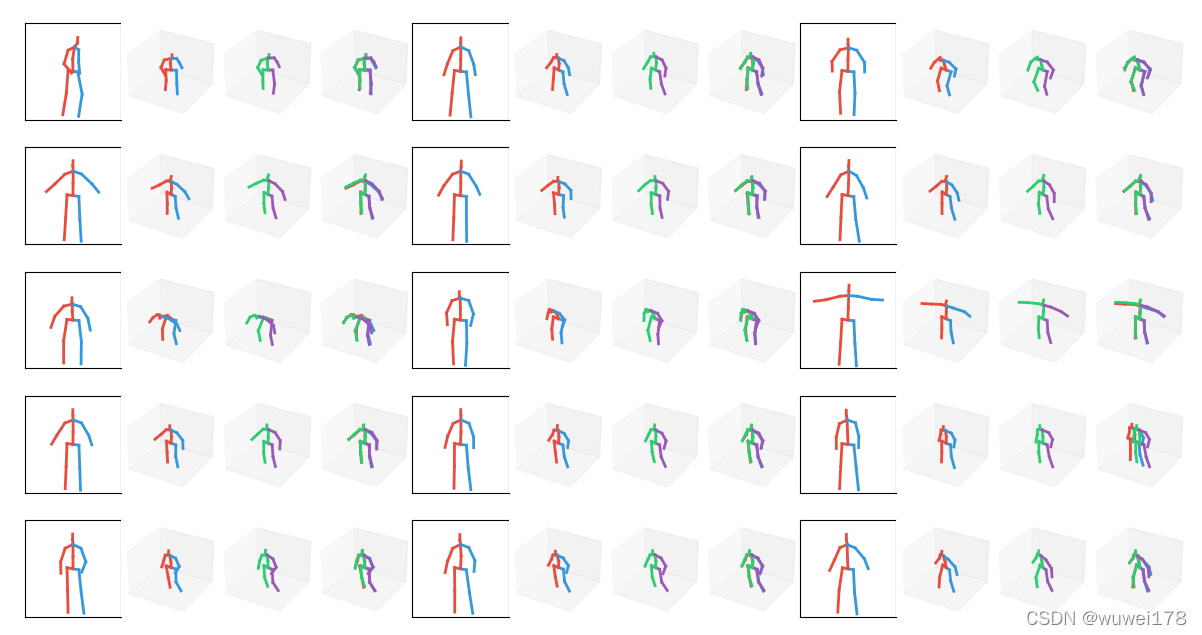
从左到右依次是2D的、预测的、真实的和预测真实合并的。


 1424
1424

 被折叠的 条评论
为什么被折叠?
被折叠的 条评论
为什么被折叠?
 到【灌水乐园】发言


