batchsize大小对卷积神经网络的影响

我们知道，batchsize是指进行一次参数学习所使用的样本数量，而iter是指所有的训练样本进入到模型中一次。那么为什么要使用batchsize呢？假如我们有几万个或几十万个数据，如果我们一下子全部读入内存的话，可能会导致溢出，毕竟计算机的内存也是有限的。但是如果一个一个样本训练的话，又会使训练时间变得很长因此合理的设置批训练样本数，是个折中的选择，那么batchsize的大小对我们的训练又有什么影响呢？

下面我用一组实验来看一下效果。

采用TensorFlow的二维卷积神经网络实现MNIST数据集的的数字识别，网络结构为1个卷积层和2个全连接层

代码如下：

#2021.11.10 HIT ATCI LZH
#batchsize大小对卷积神经网络的影响，TensorFlow二维卷积神经网络实现MNIST数据集的的数字识别，网络结构为1个卷积层和2个全连接层
#从mnist中选取一部分样本
from __future__ import division,print_function#python2中也能使用python3的函数
import tensorflow as tf
import matplotlib.pyplot as plt
import numpy as np #矩阵操作库
#Import MNIST data
from tensorflow.examples.tutorials.mnist import input_data
mnist = input_data.read_data_sets("MNIST_data/",one_hot = True)
#从训练集中选取前num个数据
def train_size(num):
    print('Total Training Image in Dataset = '+
    str(mnist.train.images.shape))
    print('-----------------------------------')
    x_train = mnist.train.images[:num,:]
    print('x_train Examples Loaded = ' + str(x_train.shape))
    y_train = mnist.train.labels[:num,:]
    print('y_train Examples Loaded = ' + str(y_train.shape))
    print('')
    return x_train,y_train
#从测试集中选取前num个数据
def test_size(num):
    print('Total Test Examples in Dataset = '+
    str(mnist.test.images.shape))
    print('-----------------------------------')
    x_test = mnist.test.images[:num,:]
    print('x_test Examples Loaded =' + str(x_test.shape))
    y_test = mnist.test.labels[:num,:]
    print('y_test Examples Loaded =' + str(y_test.shape))
    return x_test,y_test
#显示训练集中的第num个数据，以图片的形式显示
def display_digit(num):
    print(y_train[num])
    label = y_train[num].argmax(axis = 0)#返回最大值索引值，也即是该数字大小
    images = x_train[num].reshape([28,28])
    plt.title('Example: %d Label: %d'%(num ,label))#显示随机读取的图片的编号
    plt.imshow(images,cmap = plt.get_cmap('gray_r'))
    plt.show()
#显示训练集中第start~stop的数据，每一列代表一个样本
def display_mult_flat(start,stop):
    images = x_train[start].reshape([1,784])
    for i in range(start+1,stop):  #进行拼接
        images = np.concatenate((images,
        x_train[i].reshape([1,784])))
    print(images.shape)
    plt.imshow(images, cmap = plt.get_cmap('gray_r'))
    plt.show()

x_train,y_train = train_size(55000)#训练集数据选取55000个
#display_digit(np.random.randint(0,x_train.shape[0]))#随机读取一张照片
#display_mult_flat(0,400)#显示0-400张图片
#parameters
learning_rate = 0.001
training_iters = 500  #训练次数
batch_size = 128 #批训练样本大小
display_step = 10
#Network Parameters
n_input = 784
# MNIST data input(img shape : 28*28)
n_classes = 10
# MNIST total classes(0-9 digitals)
dropout = 0.85
#Dropout,probalility to keep units
x = tf.placeholder(tf.float32,[None,n_input])
y = tf.placeholder(tf.float32,[None,n_classes])
keep_prob = tf.placeholder(tf.float32)
#定义一个输入为x，权值为w，偏置为b，给定步幅的卷积层，激活函数是ReLu，padding设为SAMEM模式
def conv2d(x, w, b, strides=1):
    x = tf.nn.conv2d(x, w, strides = [1, strides, strides, 1],
        padding = 'SAME')
    x = tf.nn.bias_add(x,b)
    return tf.nn.relu(x)
#定义一个输入是x的maxpool层，卷积核为ksize并且padding为SAME
def maxpool2d(x, k=2):
    return tf.nn.max_pool(x, ksize = [1, k, k, 1],strides = [1, k, k, 1],
            padding = 'SAME')
#定义卷积神经网络，其构成是两个卷积层，一个droup层，最后是输出层
def conv_net(x, weights, biases, dropout):
    #reshape the input picture
    x = tf.reshape(x, shape = [-1, 28, 28, 1])#用于将读取的MNIST数据集的向量形式转变为图片形式，784=28*28
    #First convolution layer
    conv1 = conv2d(x, weights['wc1'], biases['bc1'])
    #Max Pooling used for downingsampling
    conv1 = maxpool2d(conv1, k=2)
    fc1 = tf.reshape(conv1, [-1,
    weights['wd1'].get_shape().as_list()[0]])
    #Fully connected layer
    fc1 = tf.add(tf.matmul(fc1, weights['wd1']),biases['bd1'])
    fc1 = tf.nn.relu(fc1)
    out = tf.add(tf.matmul(fc1,weights['out']),biases['out'])
    return out
#定义网络层的权重和偏置，第一个conv层有一个5*5的卷积核，一个输入和32个输出。第二个
#conv层有1个5*5的卷积核，32个输入和64个输出。全连接层有1024个输入和10个输出对应于最后
#的数字数目。所有的权重和偏置用randon_normal分布完成初始化：
weights = {
    #5*5 conv ,1 input, and 32 outputs
    'wc1':tf.Variable(tf.random_normal([5, 5, 1, 32])),
    # fully connected, 7*7*64 inputs, and 1024 outputs
    'wd1':tf.Variable(tf.random_normal([14*14*32, 500])),
    'out':tf.Variable(tf.random_normal([500, n_classes]))
}
biases = {
    'bc1':tf.Variable(tf.random_normal([32])),
    'bc2':tf.Variable(tf.random_normal([64])),
    'bd1':tf.Variable(tf.random_normal([500])),
    'out':tf.Variable(tf.random_normal([n_classes]))
  }
#建立一个给定权重和偏置的convnet。定义基于cross_entropy_with_logits的损失函数，并用Adam优化器进行损失最小化。
#优化后，计算精度：
pred = conv_net(x, weights, biases, keep_prob)
cost = tf.reduce_mean(tf.nn.softmax_cross_entropy_with_logits(
    logits = pred, labels = y))
optimizer = tf.train.AdamOptimizer(learning_rate = learning_rate).minimize(cost)
correct_prediction = tf.equal(tf.argmax(pred,1),tf.argmax(y,1))
accuray = tf.reduce_mean(tf.cast(correct_prediction,tf.float32))
init = tf.global_variables_initializer()
#启动计算图，并迭代train_iterats次，其中每次输入batch_size个数据进行优化，请注意，用从mnist数据集分离出的
#mnist.train数据进行训练，每进行display_step次迭代，会计算当前的精度，最后，在2048个测试图片上计算精度，
#此时无dropout
train_loss = []
train_acc = []
test_acc = []
with tf.Session() as sess:
    sess.run(init)
    step = 1
    while step <= training_iters:
        batch_x, batch_y = mnist.train.next_batch(batch_size)
        sess.run(optimizer, feed_dict = {x: batch_x, y:batch_y,
                                         keep_prob: dropout})
        if step % display_step == 0:
            loss_train, acc_train = sess.run([cost, accuray],
                                         feed_dict = {x:batch_x,
                                                      y:batch_y,
                                                      keep_prob:1.})
            print("Iter" + str(step) + ",Minibatch Loss = " + "{:.2f}".format(loss_train) +\
                ", Training Accuracy = {:.2f}".format(acc_train))
            #Calculate accuray for 2048 mnist test images.
            #Note that in this case no dropout
            acc_test = sess.run(accuray, feed_dict = {x: mnist.test.images,
                                                  y: mnist.test.labels,
                                                  keep_prob: 1.})
            print("Testing Accuracy: {:.2f}".format(acc_test))
            train_loss.append(loss_train)
            train_acc.append(acc_train)
            test_acc.append(acc_test)
        step  += 1
eval_indices = range(0, training_iters, display_step)
#Plot loss over time
plt.plot(eval_indices, train_loss, 'k-')
plt.title("Softmax Loss per iteration, batchsize = 128")
plt.xlabel("Iteration")
plt.ylabel("Softmax Loss")
plt.show()
#Plot train and test accuracy
plt.plot(eval_indices, train_acc, 'k--',label = "Train Set Accuracy")
plt.plot(eval_indices, test_acc, 'r--',label = "Test Set Accuracy")
plt.title("Train and Test Accuracy, batchsize = 128")
plt.xlabel("Genetation")
plt.ylabel("Accuracy")
plt.legend(loc = "lower right")
plt.show()

1、batchsize = 128

看一下结果：

我们可以看到当batchsizr = 128的时候，softmax loss值随着iteration的增加在不断变小，但是有一定的波动，训练集的准确率在不断波动，Test测试集的准确率不断增大，相对平缓。 

2、batchsize = 256

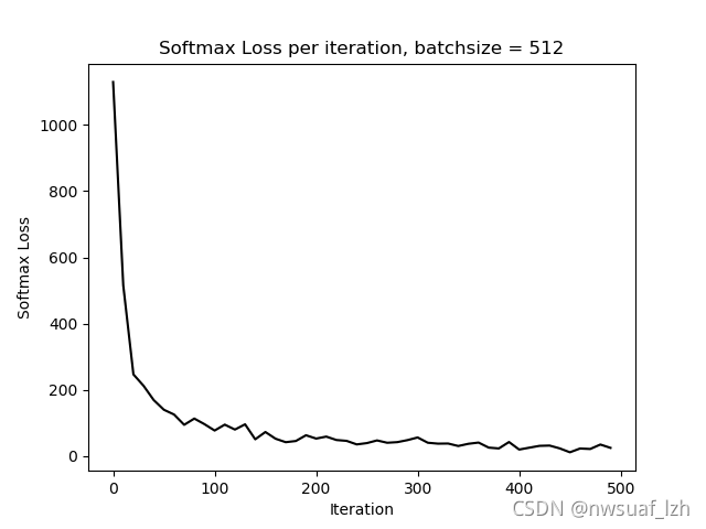
3、batchsize = 512

下面我们增大batchsize至512 

 

4、batchsize = 1024

下面我们来个更狠的

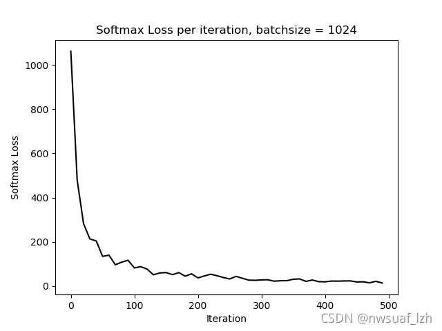
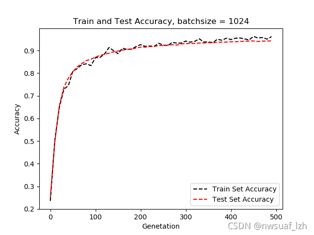
 由以上结果我们可以知道，随着batchsize的增大，准确率和softmax loss会变得平缓，但是batchsize越大的话，对内存的占用也会越大。

我看到过一种方法，batchsize就等于所有的样本数。