动手入门深度学习笔记-CNN模型以及进阶模型

CNN模型

code实现

## 二维互相关
import torch 
import torch.nn as nn

def corr2d(X, K):
    H, W = X.shape
    h, w = K.shape
    Y = torch.zeros(H - h + 1, W - w + 1)
    for i in range(Y.shape[0]):
        for j in range(Y.shape[1]):
            Y[i, j] = (X[i: i + h, j: j + w] * K).sum()
    return Y

X = torch.tensor([[0, 1, 2], [3, 4, 5], [6, 7, 8]])
K = torch.tensor([[0, 1], [2, 3]])
Y = corr2d(X, K)
print(Y)

## 二维卷积层
#二维卷积层将输入和卷积核做互相关运算，并加上一个标量偏置来得到输出。卷积层的模型参数包括卷积核和标量偏置
class Conv2D(nn.Module):
    def __init__(self, kernel_size):
        super(Conv2D, self).__init__()
        self.weight = nn.Parameter(torch.randn(kernel_size))
        self.bias = nn.Parameter(torch.randn(1))

    def forward(self, x):
        return corr2d(x, self.weight) + self.bias

## 例子
X = torch.ones(6, 8)
Y = torch.zeros(6, 7)
X[:, 2: 6] = 0
Y[:, 1] = 1
Y[:, 5] = -1
print(X)
print(Y)

conv2d = Conv2D(kernel_size =(1,2))
step = 30
lr = 0.01
for i in range(step):
    Y_hat = conv2d(X)
    l = ((Y_hat - Y)**2).sum()
    l.backward()
    # 梯度下降
    conv2d.weight.data -= lr * conv2d.weight.grad
    conv2d.bias.data -= lr * conv2d.bias.grad
        # 梯度清零
    conv2d.weight.grad.zero_()
    conv2d.bias.grad.zero_()
    if (i + 1) % 5 == 0:
        print('Step %d, loss %.3f' % (i + 1, l.item()))

print(conv2d.weight.data)
print(conv2d.bias.data)

## 将核数组上下翻转，左右翻转 在与输入组做互相关运算 这一过程叫做卷积运算

## 特征图与感受野定义
"""
二维卷积层输出的二维数组可以看作是输入在空间维度（宽和高）上某一级的表征，
也叫特征图（feature map）。影响元素的前向计算的所有可能输入区域
(可能大于输入的实际尺寸）叫做的感受野（receptive field）
"""
### 填充和步幅
"""
填充指的是在输入高和宽的两侧填充元素
步幅:卷积和在输入数组上滑动 每次滑动的行数与列数即为步幅
"""

## 多输入通道和多输出通道
"""
我们将大小为3的这一维称为通道维
"""
## 二维卷积层与全连接层对比
"""
二维卷积层常用于处理图像有两个优势
1:全连接层把图像展平成一个向量 在输入图像上相邻的元素可能因为展平操作不再相邻 网络难以捕捉局部信息
而卷积层的设计 天然地具有提取局部信息的能力
2:卷积层的参数量更少
"""
X = torch.rand(4,2,3,5)
print(X.shape)

conv2d = nn.Conv2d(in_channels = 2,out_channels = 3,kernel_size=(3,5),stride = 1,padding = (1,2))
Y = conv2d(X)
print('Y.shape: ', Y.shape)
print('weight.shape: ', conv2d.weight.shape)
print('bias.shape: ', conv2d.bias.shape)

## 池化
"""
池化层主要是计算池化窗口内元素的最大值或平均值
池化层的输出通道道数和输入通道数相等
"""
X = torch.arange(32, dtype=torch.float32).view(1, 2, 4, 4)
pool2d = nn.MaxPool2d(kernel_size=3, padding=1, stride=(2, 1))
Y = pool2d(X)
print(X)
print(Y)

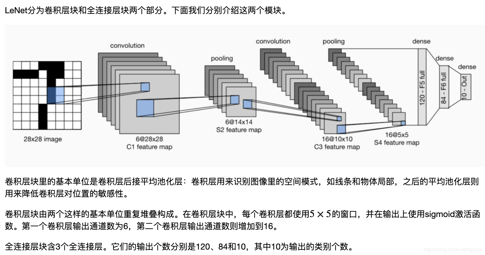
LeNet模型

1.模型框架

2.code 实现

## 二维互相关
import torch 
import torch.nn as nn

def corr2d(X, K):
    H, W = X.shape
    h, w = K.shape
    Y = torch.zeros(H - h + 1, W - w + 1)
    for i in range(Y.shape[0]):
        for j in range(Y.shape[1]):
            Y[i, j] = (X[i: i + h, j: j + w] * K).sum()
    return Y

X = torch.tensor([[0, 1, 2], [3, 4, 5], [6, 7, 8]])
K = torch.tensor([[0, 1], [2, 3]])
Y = corr2d(X, K)
print(Y)

## 二维卷积层
#二维卷积层将输入和卷积核做互相关运算，并加上一个标量偏置来得到输出。卷积层的模型参数包括卷积核和标量偏置
class Conv2D(nn.Module):
    def __init__(self, kernel_size):
        super(Conv2D, self).__init__()
        self.weight = nn.Parameter(torch.randn(kernel_size))
        self.bias = nn.Parameter(torch.randn(1))

    def forward(self, x):
        return corr2d(x, self.weight) + self.bias

## 例子
X = torch.ones(6, 8)
Y = torch.zeros(6, 7)
X[:, 2: 6] = 0
Y[:, 1] = 1
Y[:, 5] = -1
print(X)
print(Y)

conv2d = Conv2D(kernel_size =(1,2))
step = 30
lr = 0.01
for i in range(step):
    Y_hat = conv2d(X)
    l = ((Y_hat - Y)**2).sum()
    l.backward()
    # 梯度下降
    conv2d.weight.data -= lr * conv2d.weight.grad
    conv2d.bias.data -= lr * conv2d.bias.grad
        # 梯度清零
    conv2d.weight.grad.zero_()
    conv2d.bias.grad.zero_()
    if (i + 1) % 5 == 0:
        print('Step %d, loss %.3f' % (i + 1, l.item()))

print(conv2d.weight.data)
print(conv2d.bias.data)

## 将核数组上下翻转，左右翻转 在与输入组做互相关运算 这一过程叫做卷积运算

## 特征图与感受野定义
"""
二维卷积层输出的二维数组可以看作是输入在空间维度（宽和高）上某一级的表征，
也叫特征图（feature map）。影响元素的前向计算的所有可能输入区域
(可能大于输入的实际尺寸）叫做的感受野（receptive field）
"""
### 填充和步幅
"""
填充指的是在输入高和宽的两侧填充元素
步幅:卷积和在输入数组上滑动 每次滑动的行数与列数即为步幅
"""

## 多输入通道和多输出通道
"""
我们将大小为3的这一维称为通道维
"""
## 二维卷积层与全连接层对比
"""
二维卷积层常用于处理图像有两个优势
1:全连接层把图像展平成一个向量 在输入图像上相邻的元素可能因为展平操作不再相邻 网络难以捕捉局部信息
而卷积层的设计 天然地具有提取局部信息的能力
2:卷积层的参数量更少
"""
X = torch.rand(4,2,3,5)
print(X.shape)

conv2d = nn.Conv2d(in_channels = 2,out_channels = 3,kernel_size=(3,5),stride = 1,padding = (1,2))
Y = conv2d(X)
print('Y.shape: ', Y.shape)
print('weight.shape: ', conv2d.weight.shape)
print('bias.shape: ', conv2d.bias.shape)

## 池化
"""
池化层主要是计算池化窗口内元素的最大值或平均值
池化层的输出通道道数和输入通道数相等
"""
X = torch.arange(32, dtype=torch.float32).view(1, 2, 4, 4)
pool2d = nn.MaxPool2d(kernel_size=3, padding=1, stride=(2, 1))
Y = pool2d(X)
print(X)
print(Y)

一些进阶模型介绍

1. 模型框架图

code实现

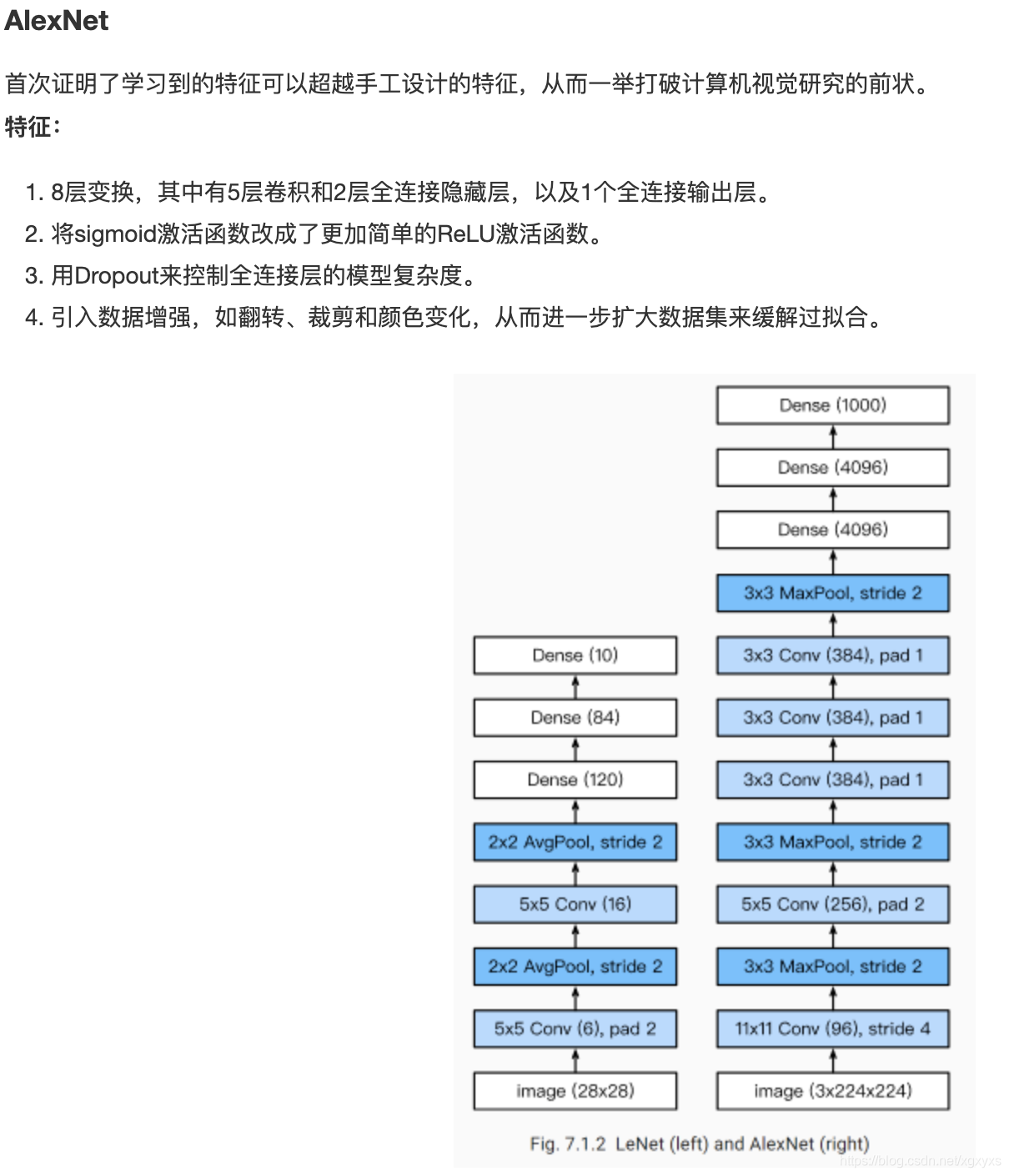
## AlexNet 神经网络
"""
特点：
8层变换，其中有5层卷积和2层全连接隐藏层，以及1个全连接输出层。
将sigmoid激活函数改成了更加简单的ReLU激活函数。
用Dropout来控制全连接层的模型复杂度。
引入数据增强，如翻转、裁剪和颜色变化，从而进一步扩大数据集来缓解过拟合。
"""
import time
import torch
from torch import nn, optim
import torchvision
import numpy as np
import sys
sys.path.append("/home/kesci/input/") 
import d2lzh1981 as d2l
import os
import torch.nn.functional as F

device = torch.device('cuda' if torch.cuda.is_available() else 'cpu')

class AlexNet(nn.Module):
    def __init__(self):
        super().__init__()
        self.conv = nn.Sequential(
            nn.Conv2d(1,96,11,4),
            nn.ReLU(),
            nn.MaxPool2d(3,2),
            ## 减少卷积窗口 使用填充为2来使得输入与输出的高和宽的一致 且增大输出通道数
            nn.Conv2d(96,256,5,1,2),
            nn.ReLU(),
            nn.MaxPool2d(3,2),
            ## 使用连续3个卷积层，且使用更小的卷积窗口，除了最后的卷积层外 进一步增大了输出通道数
            ## 前2个卷积层后不使用池化层来减小输入的高和宽
            nn.Conv2d(256,384,3,1,1),
            nn.ReLU(),
            nn.Conv2d(384,384,3,1,1),
            nn.ReLU(),
            nn.Conv2d(384,256,3,1,1),
            nn.MaxPool2d(3,2)
        )
        ## 这里全连接层的输出个数比LeNet中的大数据 使用丢弃层来缓解过拟合
        self.fc = nn.Sequential(
            nn.Linear(256*5*5,4096),
            nn.ReLU(),
            nn.Dropout(0.5),
            nn.Linear(4096,10),
        )
    def forward(self,img):
        feature = self.conv(img)
        output = self.fc(feature.view(img.shape[0],-1))
        return output
    
net = AlexNet()
print(net)

## 载入数据集
def load_data_fashion_mnist(batch_size, resize=None, root='/home/kesci/input/FashionMNIST2065'):
    """Download the fashion mnist dataset and then load into memory."""
    trans = []
    if resize:
        trans.append(torchvision.transforms.Resize(size=resize))
    trans.append(torchvision.transforms.ToTensor())
    
    transform = torchvision.transforms.Compose(trans)
    mnist_train = torchvision.datasets.FashionMNIST(root=root, train=True, download=True, transform=transform)
    mnist_test = torchvision.datasets.FashionMNIST(root=root, train=False, download=True, transform=transform)

    train_iter = torch.utils.data.DataLoader(mnist_train, batch_size=batch_size, shuffle=True, num_workers=2)
    test_iter = torch.utils.data.DataLoader(mnist_test, batch_size=batch_size, shuffle=False, num_workers=2)

    return train_iter, test_iter

#batchsize=128
batch_size = 16
# 如出现“out of memory”的报错信息，可减小batch_size或resize
train_iter, test_iter = load_data_fashion_mnist(batch_size,224)
for X, Y in train_iter:
    print('X =', X.shape,
        '\nY =', Y.type(torch.int32))
    break
r, num_epochs = 0.001, 3
optimizer = torch.optim.Adam(net.parameters(), lr=lr)
d2l.train_ch5(net, train_iter, test_iter, batch_size, optimizer, device, num_epochs)

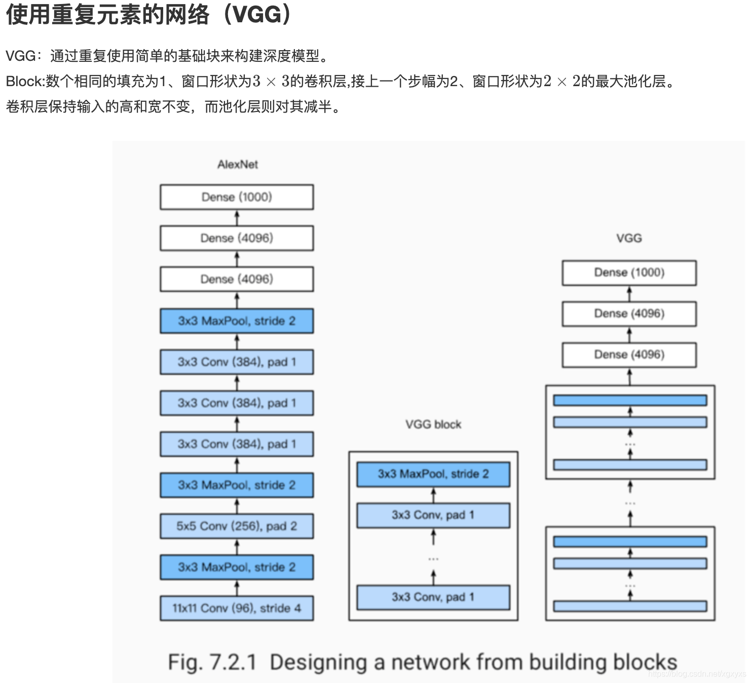
### 使用重复元素的网络VGG
"""
VGG：通过重复使⽤简单的基础块来构建深度模型。
Block:数个相同的填充为1、窗口形状为的卷积层,接上一个步幅为2、窗口形状为的最大池化层。
卷积层保持输入的高和宽不变，而池化层则对其减半。
"""
## VGG11实现
def vgg_block(num_convs, in_channels, out_channels): #卷积层个数，输入通道数，输出通道数
    blk = []
    for i in range(num_convs):
        if i == 0:
            blk.append(nn.Conv2d(in_channels, out_channels, kernel_size=3, padding=1))
        else:
            blk.append(nn.Conv2d(out_channels, out_channels, kernel_size=3, padding=1))
        blk.append(nn.ReLU())
    blk.append(nn.MaxPool2d(kernel_size=2, stride=2)) # 这里会使宽高减半
    return nn.Sequential(*blk)

conv_arch = ((1, 1, 64), (1, 64, 128), (2, 128, 256), (2, 256, 512), (2, 512, 512))
# 经过5个vgg_block, 宽高会减半5次, 变成 224/32 = 7
fc_features = 512 * 7 * 7 # c * w * h
fc_hidden_units = 4096 # 任意
def vgg(conv_arch, fc_features, fc_hidden_units=4096):
    net = nn.Sequential()
    # 卷积层部分
    for i, (num_convs, in_channels, out_channels) in enumerate(conv_arch):
        # 每经过一个vgg_block都会使宽高减半
        net.add_module("vgg_block_" + str(i+1), vgg_block(num_convs, in_channels, out_channels))
    # 全连接层部分
    net.add_module("fc", nn.Sequential(d2l.FlattenLayer(),
                                 nn.Linear(fc_features, fc_hidden_units),
                                 nn.ReLU(),
                                 nn.Dropout(0.5),
                                 nn.Linear(fc_hidden_units, fc_hidden_units),
                                 nn.ReLU(),
                                 nn.Dropout(0.5),
                                 nn.Linear(fc_hidden_units, 10)
                                ))
    return net
net = vgg(conv_arch, fc_features, fc_hidden_units)
X = torch.rand(1, 1, 224, 224)

# named_children获取一级子模块及其名字(named_modules会返回所有子模块,包括子模块的子模块)
for name, blk in net.named_children(): 
    X = blk(X)
    print(name, 'output shape: ', X.shape)

ratio = 8
small_conv_arch = [(1, 1, 64//ratio), (1, 64//ratio, 128//ratio), (2, 128//ratio, 256//ratio), 
                   (2, 256//ratio, 512//ratio), (2, 512//ratio, 512//ratio)]
net = vgg(small_conv_arch, fc_features // ratio, fc_hidden_units // ratio)
print(net)
batchsize=16
#batch_size = 64
# 如出现“out of memory”的报错信息，可减小batch_size或resize
# train_iter, test_iter = d2l.load_data_fashion_mnist(batch_size, resize=224)

lr, num_epochs = 0.001, 5
optimizer = torch.optim.Adam(net.parameters(), lr=lr)
d2l.train_ch5(net, train_iter, test_iter, batch_size, optimizer, device, num_epochs)

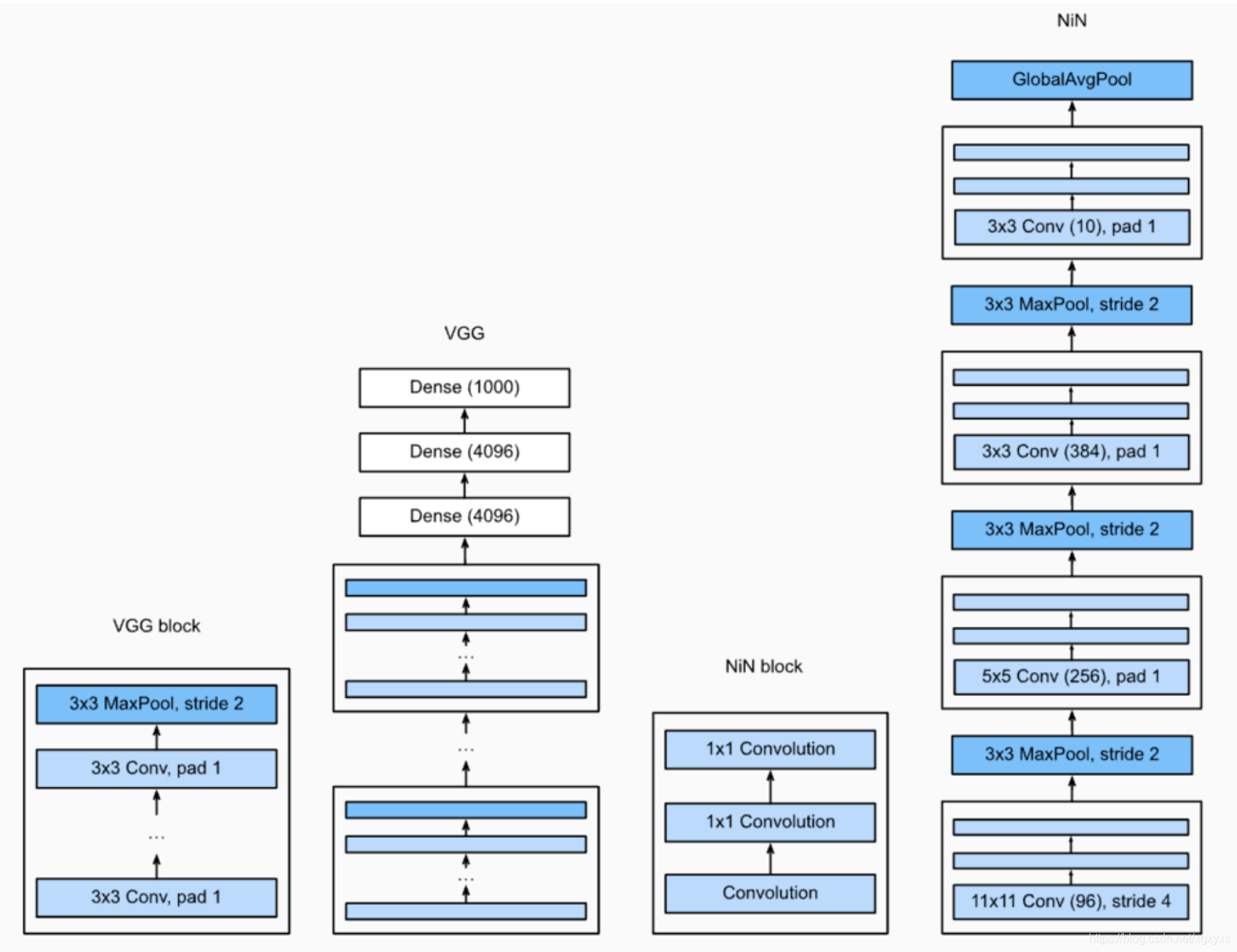
## NiN
"""
串联多个由卷积层和“全连接”层构成的小⽹络来构建⼀个深层⽹络
⽤了输出通道数等于标签类别数的NiN块，然后使⽤全局平均池化层对每个通道中所有元素求平均并直接⽤于分类
"""

##1×1卷积核作用
"""
1.放缩通道数：通过控制卷积核的数量达到通道数的放缩。
2.增加非线性。1×1卷积核的卷积过程相当于全连接层的计算过程，并且还加入了非线性激活函数，从而可以增加网络的非线性。
3.计算参数少
"""
def nin_block(in_channels, out_channels, kernel_size, stride, padding):
    blk = nn.Sequential(nn.Conv2d(in_channels, out_channels, kernel_size, stride, padding),
                        nn.ReLU(),
                        nn.Conv2d(out_channels, out_channels, kernel_size=1),
                        nn.ReLU(),
                        nn.Conv2d(out_channels, out_channels, kernel_size=1),
                        nn.ReLU())
    return blk

class GlobalAvgPool2d(nn.Module):
    # 全局平均池化层可通过将池化窗口形状设置成输入的高和宽实现
    def __init__(self):
        super(GlobalAvgPool2d, self).__init__()
    def forward(self, x):
        return F.avg_pool2d(x, kernel_size=x.size()[2:])

net = nn.Sequential(
    nin_block(1, 96, kernel_size=11, stride=4, padding=0),
    nn.MaxPool2d(kernel_size=3, stride=2),
    nin_block(96, 256, kernel_size=5, stride=1, padding=2),
    nn.MaxPool2d(kernel_size=3, stride=2),
    nin_block(256, 384, kernel_size=3, stride=1, padding=1),
    nn.MaxPool2d(kernel_size=3, stride=2), 
    nn.Dropout(0.5),
    # 标签类别数是10
    nin_block(384, 10, kernel_size=3, stride=1, padding=1),
    GlobalAvgPool2d(), 
    # 将四维的输出转成二维的输出，其形状为(批量大小, 10)
    d2l.FlattenLayer())

X = torch.rand(1, 1, 224, 224)
for name, blk in net.named_children(): 
    X = blk(X)
    print(name, 'output shape: ', X.shape)

batch_size = 128
# 如出现“out of memory”的报错信息，可减小batch_size或resize
#train_iter, test_iter = d2l.load_data_fashion_mnist(batch_size, resize=224)

lr, num_epochs = 0.002, 5
optimizer = torch.optim.Adam(net.parameters(), lr=lr)
d2l.train_ch5(net, train_iter, test_iter, batch_size, optimizer, device, num_epochs)

## NiN的优缺点
"""
NiN重复使⽤由卷积层和代替全连接层的1×1卷积层构成的NiN块来构建深层⽹络。
NiN去除了容易造成过拟合的全连接输出层，而是将其替换成输出通道数等于标签类别数 的NiN块和全局平均池化层。
NiN的以上设计思想影响了后⾯⼀系列卷积神经⽹络的设计。
"""
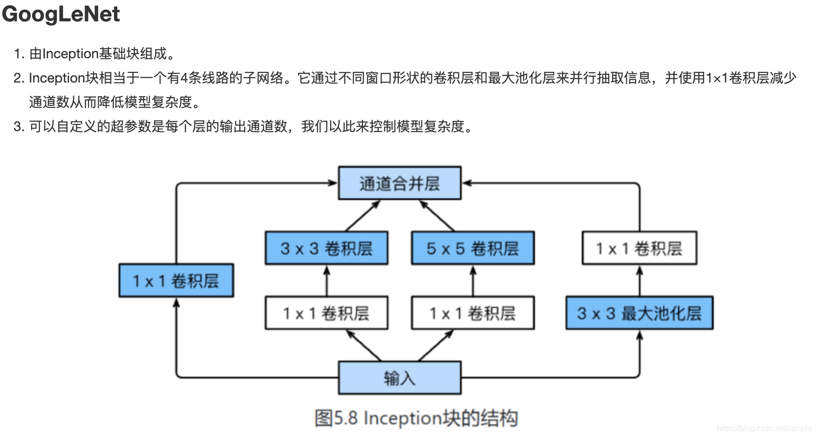
## GoogLeNet
"""
由Inception基础块组成。
Inception块相当于⼀个有4条线路的⼦⽹络。
它通过不同窗口形状的卷积层和最⼤池化层来并⾏抽取信息，并使⽤1×1卷积层减少通道数从而降低模型复杂度。
可以⾃定义的超参数是每个层的输出通道数，我们以此来控制模型复杂度。
"""
class Inception(nn.Module):
    # c1 - c4为每条线路里的层的输出通道数
    def __init__(self, in_c, c1, c2, c3, c4):
        super(Inception, self).__init__()
        # 线路1，单1 x 1卷积层
        self.p1_1 = nn.Conv2d(in_c, c1, kernel_size=1)
        # 线路2，1 x 1卷积层后接3 x 3卷积层
        self.p2_1 = nn.Conv2d(in_c, c2[0], kernel_size=1)
        self.p2_2 = nn.Conv2d(c2[0], c2[1], kernel_size=3, padding=1)
        # 线路3，1 x 1卷积层后接5 x 5卷积层
        self.p3_1 = nn.Conv2d(in_c, c3[0], kernel_size=1)
        self.p3_2 = nn.Conv2d(c3[0], c3[1], kernel_size=5, padding=2)
        # 线路4，3 x 3最大池化层后接1 x 1卷积层
        self.p4_1 = nn.MaxPool2d(kernel_size=3, stride=1, padding=1)
        self.p4_2 = nn.Conv2d(in_c, c4, kernel_size=1)

    def forward(self, x):
        p1 = F.relu(self.p1_1(x))
        p2 = F.relu(self.p2_2(F.relu(self.p2_1(x))))
        p3 = F.relu(self.p3_2(F.relu(self.p3_1(x))))
        p4 = F.relu(self.p4_2(self.p4_1(x)))
        return torch.cat((p1, p2, p3, p4), dim=1)  # 在通道维上连结输出
    
b1 = nn.Sequential(nn.Conv2d(1, 64, kernel_size=7, stride=2, padding=3),
                   nn.ReLU(),
                   nn.MaxPool2d(kernel_size=3, stride=2, padding=1))

b2 = nn.Sequential(nn.Conv2d(64, 64, kernel_size=1),
                   nn.Conv2d(64, 192, kernel_size=3, padding=1),
                   nn.MaxPool2d(kernel_size=3, stride=2, padding=1))

b3 = nn.Sequential(Inception(192, 64, (96, 128), (16, 32), 32),
                   Inception(256, 128, (128, 192), (32, 96), 64),
                   nn.MaxPool2d(kernel_size=3, stride=2, padding=1))

b4 = nn.Sequential(Inception(480, 192, (96, 208), (16, 48), 64),
                   Inception(512, 160, (112, 224), (24, 64), 64),
                   Inception(512, 128, (128, 256), (24, 64), 64),
                   Inception(512, 112, (144, 288), (32, 64), 64),
                   Inception(528, 256, (160, 320), (32, 128), 128),
                   nn.MaxPool2d(kernel_size=3, stride=2, padding=1))

b5 = nn.Sequential(Inception(832, 256, (160, 320), (32, 128), 128),
                   Inception(832, 384, (192, 384), (48, 128), 128),
                   d2l.GlobalAvgPool2d())

net = nn.Sequential(b1, b2, b3, b4, b5, 
                    d2l.FlattenLayer(), nn.Linear(1024, 10))

net = nn.Sequential(b1, b2, b3, b4, b5, d2l.FlattenLayer(), nn.Linear(1024, 10))

X = torch.rand(1, 1, 96, 96)

for blk in net.children(): 
    X = blk(X)
    print('output shape: ', X.shape)


#batchsize=128
batch_size = 16
# 如出现“out of memory”的报错信息，可减小batch_size或resize
#train_iter, test_iter = d2l.load_data_fashion_mnist(batch_size, resize=96)

lr, num_epochs = 0.001, 5
optimizer = torch.optim.Adam(net.parameters(), lr=lr)
d2l.train_ch5(net, train_iter, test_iter, batch_size, optimizer, device, num_epochs)