What is Mahalanobis distance?

Distance in standard units

In statistics, we sometimes measure "nearness" or "farness" in terms of the scale of the data. Often "scale" means "standard deviation." For univariate data, we say that an observation that is one standard deviation from the mean is closer to the mean than an observation that is three standard deviations away. (You can also specify the distance between two observations by specifying how many standard deviations apart they are.)

For many distributions, such as the normal distribution, this choice of scale also makes a statement about probability. Specifically, it is more likely to observe an observation that is about one standard deviation from the mean than it is to observe one that is several standard deviations away. Why? Because the probability density function is higher near the mean and nearly zero as you move many standard deviations away.

For normally distributed data, you can specify the distance from the mean by computing the so-called z-score. For a value x, the z-score of x is the quantity z = (x-μ)/σ, where μ is the population mean and σ is the population standard deviation. This is a dimensionless quantity that you can interpret as the number of standard deviations that x is from the mean.

Distance is not always what it seems

You can generalize these ideas to the multivariate normal distribution. The following graph shows simulated bivariate normal data that is overlaid with prediction ellipses. The ellipses in the graph are the 10% (innermost), 20%, ..., and 90% (outermost) prediction ellipses for the bivariate normal distribution that generated the data. The prediction ellipses are contours of the bivariate normal density function. The probability density is high for ellipses near the origin, such as the 10% prediction ellipse. The density is low for ellipses are further away, such as the 90% prediction ellipse.

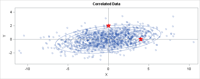
In the graph, two observations are displayed by using red stars as markers. The first observation is at the coordinates (4,0), whereas the second is at (0,2). The question is: which marker is closer to the origin? (The origin is the multivariate center of this distribution.)

The answer is, "It depends how you measure distance." The Euclidean distances are 4 and 2, respectively, so you might conclude that the point at (0,2) is closer to the origin. However, for this distribution, the variance in the Y direction is less than the variance in the X direction, so in some sense the point (0,2) is "more standard deviations" away from the origin than (4,0) is.

Notice the position of the two observations relative to the ellipses. The point (0,2) is located at the 90% prediction ellipse, whereas the point at (4,0) is located at about the 75% prediction ellipse. What does this mean? It means that the point at (4,0) is "closer" to the origin in the sense that you are more likely to observe an observation near (4,0) than to observe one near (0,2). The probability density is higher near (4,0) than it is near (0,2).

In this sense, prediction ellipses are a multivariate generalization of "units of standard deviation." You can use the bivariate probability contours to compare distances to the bivariate mean. A point p is closer than a point q if the contour that contains p is nested within the contour that contains q.

Defining the Mahalanobis distance

You can use the probability contours to define the Mahalanobis distance. The Mahalanobis distance has the following properties:

• It accounts for the fact that the variances in each direction are different.
• It accounts for the covariance between variables.
• It reduces to the familiar Euclidean distance for uncorrelated variables with unit variance.

For univariate normal data, the univariate z-score standardizes the distribution (so that it has mean 0 and unit variance) and gives a dimensionless quantity that specifies the distance from an observation to the mean in terms of the scale of the data. For multivariate normal data with mean μ and covariance matrix Σ, you can decorrelate the variables and standardize the distribution by applying the Cholesky transformation z = L-1(x - μ), where L is the Cholesky factor of Σ, Σ=LLT.

After transforming the data, you can compute the standard Euclidian distance from the point z to the origin. In order to get rid of square roots, I'll compute the square of the Euclidean distance, which is dist2(z,0) = zTz. This measures how far from the origin a point is, and it is the multivariate generalization of a z-score.

You can rewrite zTz in terms of the original correlated variables. The squared distance Mahal2(x,μ) is 
= zT z 
= (L-1(x - μ))T (L-1(x - μ)) 
= (x - μ)T (LLT)-1 (x - μ) 
= (x - μ)T Σ -1 (x - μ) 
The last formula is the definition of the squared Mahalanobis distance. The derivation uses several matrix identities such as (AB)T = BTAT, (AB)-1 = B-1A-1, and (A-1)T = (AT)-1. Notice that if Σ is the identity matrix, then the Mahalanobis distance reduces to the standard Euclidean distance between x and μ.

The Mahalanobis distance accounts for the variance of each variable and the covariance between variables. Geometrically, it does this by transforming the data into standardized uncorrelated data and computing the ordinary Euclidean distance for the transformed data. In this way, the Mahalanobis distance is like a univariate z-score: it provides a way to measure distances that takes into account the scale of the data.