Mahalanobis Distance和Euclidean Distance

马氏距离是一种有效的多元距离度量标准，用于测量点（向量）与分布之间的距离。常用在多变量异常检测，高度不平衡的数据集分类应用中。

本文解释为什么和何时用Mahalanobis Distance。

Euclidean Distance

欧几里德距离是两点之间常用的直线距离。

如果两个点都在二维平面中（也就是说，数据集中有两个数字列（）和（）），则两个点（，）和（，)之间的欧式距离 ）是：

该公式可以扩展到所需的任意多个维度：

当数据点可均等加权且彼此独立，欧几里得距离就可以正常工作。

让我们考虑一个例子，如下表：

上面的两个表格显示了相同对象的“面积”和“价格”。 仅变量的单位改变。

由于两个表都表示相同的实体，因此任意两行（点A和点B）之间的距离都应该相同。 但是，即使在物理空间上，距离是相同的，欧几里得距离也给出了不同的值。

从技术上讲，可以通过缩放变量，计算z分数（例如：（x –平均值）/ std）或使其在特定范围内（例如：归一化）变化来克服。

但是还有另一个主要缺点。

也就是说，如果维度（数据集中的列）相互关联（这在实际数据集中通常是这种情况），则对于测量一点实际上离集群有多近，点与点中心（分布）之间的欧几里得距离所给出的信息很少或具有误导性。

如果和是不相关的，与中心点的欧几里得距离，可以用于辨别是否是内部成员。

如果和是不相关的。Point 1和点2与中心点的欧几里得距离相同，但是Point 1属于分布，Point 2是离群点。为了检测Point 2是离群点，Point 1与中心点的距离应该大于Point 2 与中心点的距离。

这是因为，欧几里得距离仅是两点之间的距离。 它不考虑数据集中的其余点如何变化。 因此，它不能真正用来判断一个点实际上与点的分布有多接近。

这里我们需要的是更健壮的距离度量标准，该度量标准可以精确表示一个点距分布的距离。

Mahalanobis Distance

马氏距离是点与分布之间的距离。 并且不在两个不同的点之间。 它实际上是欧几里得距离的多元等效项。

它是由P. C. Mahalanobis教授于1936年提出的，此后一直在各种统计应用中使用。 但是，它在机器学习实践中并不为人所知或使用。

那么从计算上来说，马氏距离与欧几里得距离有何不同？

• Mahalanobis Distance将列转换为不相关的变量
• 缩放列以使其方差等于1
• 最后，Mahalanobis Distance计算出欧几里得距离

计算马氏距离的公式如下：

• 是马氏距离的平方；
• 是观测值的向量（数据集中的行）；
• 是自变量平均值的向量（每列的平均值）；
• 是自变量的逆协方差矩阵。

本质上是向量与平均值的距离。 然后，将其除以协方差矩阵（或乘以协方差矩阵的逆数）。

考虑一下，这实际上是常规标准化的多元变量（）。 也就是说，=（向量）–（平均向量）/（协方差矩阵）。

那么，除以协方差的作用是什么？

如果数据集中的变量高度相关，则协方差将很高。 除以较大的协方差将有效地减小距离。

同样，如果X不相关，则协方差也不大，距离也不会减少太多。

因此，Mahalanobis Distance有效地解决了规模问题以及谈到的变量之间的相关性。

 Mahalanobis Distance in Python

import pandas as pd
import scipy as sp
import numpy as np

filepath = 'https://raw.githubusercontent.com/selva86/datasets/master/diamonds.csv'
df = pd.read_csv(filepath).iloc[:, [0,4,6]]
print(df.head())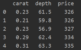

def mahalanobis(x=None, data=None, cov=None):
    """Compute the Mahalanobis Distance between each row of x and the data  
    x    : vector or matrix of data with, say, p columns.
    data : ndarray of the distribution from which Mahalanobis distance of each observation of x is to be computed.
    cov  : covariance matrix (p x p) of the distribution. If None, will be computed from data.
    """
    x_minus_mu = x - np.mean(data)
    if not cov:
        cov = np.cov(data.values.T)
    inv_covmat = np.linalg.inv(cov)
    left_term = np.dot(x_minus_mu, inv_covmat)
    mahal = np.dot(left_term, x_minus_mu.T)
    return mahal.diagonal()


df_x = df[['carat', 'depth', 'price']].head(500)
df_x['mahala'] = mahalanobis(x=df_x, data=df[['carat', 'depth', 'price']])
print(df_x.head())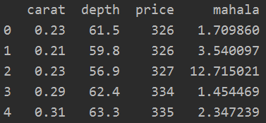

使用马氏距离的多元离群值检测

假设检验统计量遵循卡方分布，自由度为“ ”，则在0.01显着性水平和2自由度下的临界值计算如下：

# Critical values for two degrees of freedom
from scipy.stats import chi2

chi2.ppf((1-0.01), df=2)
#> 9.21

这意味着，如果观测值的马氏距离超过9.21，则可以认为是极端。

如果更喜欢P值来确定观察值是否为极值，则可以按以下方式计算P值：

# Compute the P-Values
df_x['p_value'] = 1 - chi2.cdf(df_x['mahala'], 2)

# Extreme values with a significance level of 0.01
print(df_x.loc[df_x.p_value < 0.01].head(10))

如果将上述观察值与数据集的其余部分进行比较，则显然是极端的。

Mahalanobis Distance for Classification Problems

马氏距离可用于分类问题。 Mahalanobis分类器简单实现在下面编码。 直觉是，根据马哈拉诺比斯距离，将观察值分配给与其最接近的类别。

看一下BreastCancer数据集上实现的示例，其目的是确定肿瘤是良性还是恶性的。

df = pd.read_csv('https://raw.githubusercontent.com/selva86/datasets/master/BreastCancer.csv',
                 usecols=['Cl.thickness', 'Cell.size', 'Marg.adhesion',
                          'Epith.c.size', 'Bare.nuclei', 'Bl.cromatin', 'Normal.nucleoli',
                          'Mitoses', 'Class'])

df.dropna(inplace=True)  # drop missing values.
print(df.head())

以7:3的比例将数据集拆分为训练和测试。 然后将训练数据集分为“ pos”（1）和“ neg”（0）类的同类组。 为了预测测试数据集的类别，我们测量给定观测值（行）与正值数据集（xtrain_pos）和负值数据集（xtrain_neg）之间的马氏距离。 

然后，根据观察到的最接近的组为其分配类别。

from sklearn.model_selection import train_test_split
xtrain, xtest, ytrain, ytest = train_test_split(df.drop('Class', axis=1), df['Class'], test_size=.3, random_state=100)

# Split the training data as pos and neg
xtrain_pos = xtrain.loc[ytrain == 1, :]
xtrain_neg = xtrain.loc[ytrain == 0, :]

构建MahalanobiBinaryClassifier。 为此，需要定义predict_proba（）和predict（）方法。 此分类器不需要单独的fit（）（训练）方法。

class MahalanobisBinaryClassifier():
    def __init__(self, xtrain, ytrain):
        self.xtrain_pos = xtrain.loc[ytrain == 1, :]
        self.xtrain_neg = xtrain.loc[ytrain == 0, :]

    def predict_proba(self, xtest):
        pos_neg_dists = [(p,n) for p, n in zip(mahalanobis(xtest, self.xtrain_pos), mahalanobis(xtest, self.xtrain_neg))]
        return np.array([(1-n/(p+n), 1-p/(p+n)) for p,n in pos_neg_dists])

    def predict(self, xtest):
        return np.array([np.argmax(row) for row in self.predict_proba(xtest)])


clf = MahalanobisBinaryClassifier(xtrain, ytrain)        
pred_probs = clf.predict_proba(xtest)
pred_class = clf.predict(xtest)

# Pred and Truth
pred_actuals = pd.DataFrame([(pred, act) for pred, act in zip(pred_class, ytest)], columns=['pred', 'true'])
print(pred_actuals[:5])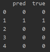        

分类器如何在测试数据集上执行

from sklearn.metrics import classification_report, accuracy_score, roc_auc_score, confusion_matrix
truth = pred_actuals.loc[:, 'true']
pred = pred_actuals.loc[:, 'pred']
scores = np.array(pred_probs)[:, 1]
print('AUROC: ', roc_auc_score(truth, scores))
print('\nConfusion Matrix: \n', confusion_matrix(truth, pred))
print('\nAccuracy Score: ', accuracy_score(truth, pred))
print('\nClassification Report: \n', classification_report(truth, pred))