回归----多元线性回归

目录

多元线性回归

 梯度下降法实现

 sklearn ---多元线性回归

---

多元线性回归

当Y值的影响因素不是唯一时，采用多元线性回归

参数： 

代价函数：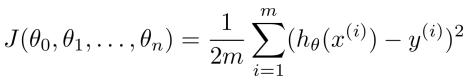

梯度下降法：

 更新参数：

 梯度下降法实现

• 首先把需要用到的库导入

import numpy as np
from numpy import genfromtxt
import matplotlib.pyplot as plt
from mpl_toolkits.mplot3d import Axes3D
%matplotlib inline

•  载入数据

#载入数据
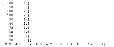
data = np.genfromtxt("Delivery.csv",delimiter=",")
print(data)

x_data = data[:,:-1]  #取全部行，不包含最后一列的数据
y_data = data[:,-1]  #取最后一列中所有行的数据
print(x_data)
print(y_data)

 载入的数据打印如第一张图，经过数据处理，打印如第二张图：

•  接下来实现最小二乘法函数以及梯度下降法的函数，更新回归线的参数，使误差更小（这里最小二乘法以及梯度下降法与一元线性回归用到的方法一样）

#学习率
lr = 0.0001
#参数
theta0 = 0
theta1 = 0
theta2 = 0
#迭代次数
epochs = 1000

#最小二乘法
def minimum_squares(x_data,y_data,theta0,theta1,theta2):
    totalError =0
    for i in range(0,len(x_data)):
        totalError += (y_data[i] -(x_data[i,0]*theta1 + x_data[i,1]*theta2 + theta0)) **2 
    return totalError / float(len(x_data))

def gradient_descent_runner(x_data,y_data,theta0,theta1,theta2,lr,epochs):
    #计算总数据量
    m = float(len(x_data))
    #循环epochs次
    for i in range (epochs):
        #设置临时量
        theta0_grad = 0
        theta1_grad = 0
        theta2_grad = 0
        
        #计算梯度总合再求平均
        for j in range (0,len(x_data)):
            theta0_grad += (1/m) *((x_data[j,0]*theta1 + x_data[j,1]*theta2 +theta0) - y_data[j])
            theta1_grad += (1/m) *((x_data[j,0]*theta1 + x_data[j,1]*theta2 +theta1) - y_data[j]) * x_data[j,0]
            theta2_grad += (1/m) *((x_data[j,0]*theta1 + x_data[j,1]*theta2 +theta2) - y_data[j]) * x_data[j,1]
            
        #更新theta0,theta1,theta2的值
        theta0 = theta0 - (lr*theta0_grad)
        theta1 = theta1 - (lr*theta1_grad)
        theta2 = theta2 - (lr*theta2_grad)
        
    return theta0,theta1,theta2

• 最后打印出结果： 

print("Staring theta0 = {0},theta1 = {1},theta2 = {2},error = {3}".
      format(theta0,theta1,theta2,minimum_squares(x_data,y_data,theta0,theta1,theta2)))
print("Running.......")
theta0,theta1,theta2 = gradient_descent_runner(x_data,y_data,theta0,theta1,theta2,lr,epochs)
print("After {0} iterations theta0 = {1},theta1 = {2},theta2 = {3},error = {4}".
      format(epochs,theta0,theta1,theta2,minimum_squares(x_data,y_data,theta0,theta1,theta2))) 

 上图是打印出来的结果，可以看出，在没有进行梯度下降前，我们得到的误差为47.27，经过梯度下降后，我们的误差减小到了0.7648

最后我们可以画出这个模型的图，来真实感受一下

ax = plt.figure().add_subplot(111,projection = '3d')
ax.scatter(x_data[:,0],x_data[:,1],y_data,c = 'r',marker = 'o',s = 100)
x0 = x_data[:,0]
x1 = x_data[:,1]

#生成网格矩阵
x0,x1 = np.meshgrid(x0,x1)
z = theta0 + theta1*x0 + theta2*x1

#画3D图
ax.plot_surface(x0,x1,z)
#设置坐标轴
ax.set_xlabel('Miles')
ax.set_ylabel('Num of Deliveries')
ax.set_zlabel('Time')

#显示图像
plt.show()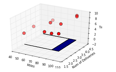

 静态的图，我们看到的并不是很清楚，但是在运行中可以将次图显示成动态的图，就可以很清楚的看到两张图误差的大小。

我用到的是jupyter，在编辑完成代码后，使用如下操作，将代码下载成python格式，然后在命令提示符中运行次代码，就可以生成动态的图。（注意在命令提示符运行中，先要将路径切换到代码存放的路径上）

 

 sklearn ---多元线性回归

其实，我们要实现多元线性回归，我们也可以直接调用库来完成，代码如下（接下来就不做解释）

from sklearn import linear_model
import numpy as np
import matplotlib.pyplot as plt
from mpl_toolkits.mplot3d import Axes3D
%matplotlib inline

#载入数据
data = np.genfromtxt("Delivery.csv",delimiter=",")
print(data)
x_data = data[:,:-1]
y_data = data[:,-1]
print(x_data)
print(y_data)

model =linear_model.LinearRegression()
model.fit(x_data,y_data)

#系数
print("coefficients:",model.coef_)
#截距
print("intercept:",model.intercept_)
#测试
x_test = [[102,4]]
predict = model.predict(x_test)
print("predict:",predict)

ax = plt.figure().add_subplot(111,projection = '3d')
ax.scatter(x_data[:,0],x_data[:,1],y_data,c = 'r',marker = 'o',s = 100)
x0 = x_data[:,0]
x1 = x_data[:,1]

#生成网格矩阵
x0,x1 = np.meshgrid(x0,x1)
z = model.intercept_ + model.coef_[0] *x0 + model.coef_[1] *x1

#画3D图
ax.plot_surface(x0,x1,z)

#设置坐标轴
ax.set_xlabel('Miles')
ax.set_ylabel('Num of Deliveries')
ax.set_zlabel('Time')

#显示图像
plt.show()

 结果如图：