cs231n：assignment2——Q2: Batch Normalization

视频里 Andrej Karpathy上课的时候说,这次的作业meaty but educational,确实很meaty,作业一般是由.ipynb文件和.py文件组成,这次因为每个.ipynb文件涉及到的.py文件较多,且互相之间有交叉,所以每篇博客只贴出一个.ipynb或者一个.py文件.(因为之前的作业由于是一个.ipynb文件对应一个.py文件,所以就整合到一篇博客里)
还是那句话,有错误希望帮我指出来,多多指教,谢谢
BatchNormalization.ipynb内容:
[TOC]

Batch Normalization

One way to make deep networks easier to train is to use more sophisticated optimization procedures such as SGD+momentum, RMSProp, or Adam. Another strategy is to change the architecture of the network to make it easier to train. One idea along these lines is batch normalization which was recently proposed by [3].

The idea is relatively straightforward. Machine learning methods tend to work better when their input data consists of uncorrelated features with zero mean and unit variance. When training a neural network, we can preprocess the data before feeding it to the network to explicitly decorrelate its features; this will ensure that the first layer of the network sees data that follows a nice distribution. However even if we preprocess the input data, the activations at deeper layers of the network will likely no longer be decorrelated and will no longer have zero mean or unit variance since they are output from earlier layers in the network. Even worse, during the training process the distribution of features at each layer of the network will shift as the weights of each layer are updated.

The authors of [3] hypothesize that the shifting distribution of features inside deep neural networks may make training deep networks more difficult. To overcome this problem, [3] proposes to insert batch normalization layers into the network. At training time, a batch normalization layer uses a minibatch of data to estimate the mean and standard deviation of each feature. These estimated means and standard deviations are then used to center and normalize the features of the minibatch. A running average of these means and standard deviations is kept during training, and at test time these running averages are used to center and normalize features.

It is possible that this normalization strategy could reduce the representational power of the network, since it may sometimes be optimal for certain layers to have features that are not zero-mean or unit variance. To this end, the batch normalization layer includes learnable shift and scale parameters for each feature dimension.

[3] Sergey Ioffe and Christian Szegedy, “Batch Normalization: Accelerating Deep Network Training by Reducing
Internal Covariate Shift”, ICML 2015.

# As usual, a bit of setup

import time
import numpy as np
import matplotlib.pyplot as plt
from cs231n.classifiers.fc_net import *
from cs231n.data_utils import get_CIFAR10_data
from cs231n.gradient_check import eval_numerical_gradient, eval_numerical_gradient_array
from cs231n.solver import Solver

%matplotlib inline
plt.rcParams['figure.figsize'] = (10.0, 8.0) # set default size of plots
plt.rcParams['image.interpolation'] = 'nearest'
plt.rcParams['image.cmap'] = 'gray'

# for auto-reloading external modules
# see http://stackoverflow.com/questions/1907993/autoreload-of-modules-in-ipython
%load_ext autoreload
%autoreload 2

def rel_error(x, y):
  """ returns relative error """
  return np.max(np.abs(x - y) / (np.maximum(1e-8, np.abs(x) + np.abs(y))))

# Load the (preprocessed) CIFAR10 data.

data = get_CIFAR10_data()
for k, v in data.iteritems():
  print '%s: ' % k, v.shape

X_val:  (1000, 3, 32, 32)
X_train:  (49000, 3, 32, 32)
X_test:  (1000, 3, 32, 32)
y_val:  (1000,)
y_train:  (49000,)
y_test:  (1000,)

Batch normalization: Forward

In the file cs231n/layers.py, implement the batch normalization forward pass in the function batchnorm_forward. Once you have done so, run the following to test your implementation.

# Check the training-time forward pass by checking means and variances
# of features both before and after batch normalization

# Simulate the forward pass for a two-layer network
N, D1, D2, D3 = 200, 50, 60, 3
X = np.random.randn(N, D1)
W1 = np.random.randn(D1, D2)
W2 = np.random.randn(D2, D3)
a = np.maximum(0, X.dot(W1)).dot(W2)

print 'Before batch normalization:'
print '  means: ', a.mean(axis=0)
print '  stds: ', a.std(axis=0)

# Means should be close to zero and stds close to one
print 'After batch normalization (gamma=1, beta=0)'
a_norm, _ = batchnorm_forward(a, np.ones(D3), np.zeros(D3), {'mode': 'train'})
print '  mean: ', a_norm.mean(axis=0)
print '  std: ', a_norm.std(axis=0)

# Now means should be close to beta and stds close to gamma
gamma = np.asarray([1.0, 2.0, 3.0])
beta = np.asarray([11.0, 12.0, 13.0])
a_norm, _ = batchnorm_forward(a, gamma, beta, {'mode': 'train'})
print 'After batch normalization (nontrivial gamma, beta)'
print '  means: ', a_norm.mean(axis=0)
print '  stds: ', a_norm.std(axis=0)

Before batch normalization:
  means:  [  9.04084554  -3.17680015  45.84413457]
  stds:  [ 28.18965752  31.76172365  30.78152211]
After batch normalization (gamma=1, beta=0)
  mean:  [ -5.96744876e-18  -1.48492330e-17  -3.33066907e-17]
  std:  [ 0.99999999  1.          0.99999999]
After batch normalization (nontrivial gamma, beta)
  means:  [ 11.  12.  13.]
  stds:  [ 0.99999999  1.99999999  2.99999998]

# Check the test-time forward pass by running the training-time
# forward pass many times to warm up the running averages, and then
# checking the means and variances of activations after a test-time
# forward pass.

N, D1, D2, D3 = 200, 50, 60, 3
W1 = np.random.randn(D1, D2)
W2 = np.random.randn(D2, D3)

bn_param = {'mode': 'train'}
gamma = np.ones(D3)
beta = np.zeros(D3)
for t in xrange(50):
  X = np.random.randn(N, D1)
  a = np.maximum(0, X.dot(W1)).dot(W2)
  batchnorm_forward(a, gamma, beta, bn_param)
bn_param['mode'] = 'test'
X = np.random.randn(N, D1)
a = np.maximum(0, X.dot(W1)).dot(W2)
a_norm, _ = batchnorm_forward(a, gamma, beta, bn_param)

# Means should be close to zero and stds close to one, but will be
# noisier than training-time forward passes.
print 'After batch normalization (test-time):'
print '  means: ', a_norm.mean(axis=0)
print '  stds: ', a_norm.std(axis=0)

After batch normalization (test-time):
  means:  [-0.11572037  0.00564579 -0.04738633]
  stds:  [ 0.96048774  0.93115169  0.88629565]

Batch Normalization: backward

Now implement the backward pass for batch normalization in the function batchnorm_backward.

To derive the backward pass you should write out the computation graph for batch normalization and backprop through each of the intermediate nodes. Some intermediates may have multiple outgoing branches; make sure to sum gradients across these branches in the backward pass.

Once you have finished, run the following to numerically check your backward pass.

# Gradient check batchnorm backward pass
# 一开始把dx求导想简单了,仔细看了计算公式才算对,一同学习的小伙伴注意这一点
# 非常详细的文章:
# https://kratzert.github.io/2016/02/12/understanding-the-gradient-flow-through-the-batch-normalization-layer.html
N, D = 4, 5
x = 5 * np.random.randn(N, D) + 12
gamma = np.random.randn(D)
beta = np.random.randn(D)
dout = np.random.randn(N, D)

bn_param = {'mode': 'train'}
fx = lambda x: batchnorm_forward(x, gamma, beta, bn_param)[0]
fg = lambda a: batchnorm_forward(x, gamma, beta, bn_param)[0]
fb = lambda b: batchnorm_forward(x, gamma, beta, bn_param)[0]

dx_num = eval_numerical_gradient_array(fx, x, dout)
da_num = eval_numerical_gradient_array(fg, gamma, dout)
db_num = eval_numerical_gradient_array(fb, beta, dout)

_, cache = batchnorm_forward(x, gamma, beta, bn_param)
dx, dgamma, dbeta = batchnorm_backward(dout, cache)

#print "dx\n",dx, "\n\ndx_num\n",dx_num

print 'dx error: ', rel_error(dx_num, dx)
print 'dgamma error: ', rel_error(da_num, dgamma)
print 'dbeta error: ', rel_error(db_num, dbeta)

dx error:  1.51270448054e-09
dgamma error:  1.17116986498e-10
dbeta error:  3.69406375577e-12

Batch Normalization: alternative backward

In class we talked about two different implementations for the sigmoid backward pass. One strategy is to write out a computation graph composed of simple operations and backprop through all intermediate values. Another strategy is to work out the derivatives on paper. For the sigmoid function, it turns out that you can derive a very simple formula for the backward pass by simplifying gradients on paper.

Surprisingly, it turns out that you can also derive a simple expression for the batch normalization backward pass if you work out derivatives on paper and simplify. After doing so, implement the simplified batch normalization backward pass in the function batchnorm_backward_alt and compare the two implementations by running the following. Your two implementations should compute nearly identical results, but the alternative implementation should be a bit faster.

NOTE: You can still complete the rest of the assignment if you don’t figure this part out, so don’t worry too much if you can’t get it.

N, D = 100, 500
x = 5 * np.random.randn(N, D) + 12
gamma = np.random.randn(D)
beta = np.random.randn(D)
dout = np.random.randn(N, D)

bn_param = {'mode': 'train'}
out, cache = batchnorm_forward(x, gamma, beta, bn_param)

t1 = time.time()
dx1, dgamma1, dbeta1 = batchnorm_backward(dout, cache)
t2 = time.time()
dx2, dgamma2, dbeta2 = batchnorm_backward_alt(dout, cache)
t3 = time.time()

print 'dx difference: ', rel_error(dx1, dx2)
print 'dgamma difference: ', rel_error(dgamma1, dgamma2)
print 'dbeta difference: ', rel_error(dbeta1, dbeta2)
print 'speedup: %.2fx' % ((t2 - t1) / (t3 - t2))

dx difference:  5.82325769318e-13
dgamma difference:  0.0
dbeta difference:  0.0
speedup: 2.09x

Fully Connected Nets with Batch Normalization

Now that you have a working implementation for batch normalization, go back to your FullyConnectedNet in the file cs2312n/classifiers/fc_net.py. Modify your implementation to add batch normalization.

Concretely, when the flag use_batchnorm is True in the constructor, you should insert a batch normalization layer before each ReLU nonlinearity. The outputs from the last layer of the network should not be normalized. Once you are done, run the following to gradient-check your implementation.

HINT: You might find it useful to define an additional helper layer similar to those in the file cs231n/layer_utils.py. If you decide to do so, do it in the file cs231n/classifiers/fc_net.py.

N, D, H1, H2, C = 2, 15, 20, 30, 10
X = np.random.randn(N, D)
y = np.random.randint(C, size=(N,))

for reg in [0, 3.14]:
  print 'Running check with reg = ', reg
  model = FullyConnectedNet([H1, H2], input_dim=D, num_classes=C,
                            reg=reg, weight_scale=5e-2, dtype=np.float64,
                            use_batchnorm=True)

  loss, grads = model.loss(X, y)
  print 'Initial loss: ', loss

  for name in sorted(grads):
    f = lambda _: model.loss(X, y)[0]
    grad_num = eval_numerical_gradient(f, model.params[name], verbose=False, h=1e-5)
    print '%s relative error: %.2e' % (name, rel_error(grad_num, grads[name]))
  if reg == 0: print

Running check with reg =  0
Initial loss:  2.37312206472
W1 relative error: 3.55e-04
W2 relative error: 4.63e-06
W3 relative error: 4.20e-09
b1 relative error: 8.74e-08
b2 relative error: 2.07e-07
b3 relative error: 1.66e-10
beta1 relative error: 1.09e-08
beta2 relative error: 3.66e-09
gamma1 relative error: 3.24e-08
gamma2 relative error: 9.31e-09

Running check with reg =  3.14
Initial loss:  6.51528528024
W1 relative error: 2.89e-06
W2 relative error: 3.09e-06
W3 relative error: 6.43e-08
b1 relative error: 8.88e-03
b2 relative error: 4.00e-07
b3 relative error: 3.66e-10
beta1 relative error: 1.49e-09
beta2 relative error: 1.38e-08
gamma1 relative error: 3.30e-09
gamma2 relative error: 3.12e-08

Batchnorm for deep networks

Run the following to train a six-layer network on a subset of 1000 training examples both with and without batch normalization.

# Try training a very deep net with batchnorm
hidden_dims = [100, 100, 100, 100, 100]

num_train = 1000
small_data = {
  'X_train': data['X_train'][:num_train],
  'y_train': data['y_train'][:num_train],
  'X_val': data['X_val'],
  'y_val': data['y_val'],
}

weight_scale = 2e-2
bn_model = FullyConnectedNet(hidden_dims, weight_scale=weight_scale, use_batchnorm=True)
model = FullyConnectedNet(hidden_dims, weight_scale=weight_scale, use_batchnorm=False)

bn_solver = Solver(bn_model, small_data,
                num_epochs=10, batch_size=50,
                update_rule='adam',
                optim_config={
                  'learning_rate': 1e-3,
                },
                verbose=True, print_every=200)
bn_solver.train()

solver = Solver(model, small_data,
                num_epochs=10, batch_size=50,
                update_rule='adam',
                optim_config={
                  'learning_rate': 1e-3,
                },
                verbose=True, print_every=200)
solver.train()

(Iteration 1 / 200) loss: 2.333149
(Epoch 0 / 10) train acc: 0.128000; val_acc: 0.141000
(Epoch 1 / 10) train acc: 0.351000; val_acc: 0.301000
(Epoch 2 / 10) train acc: 0.398000; val_acc: 0.301000
(Epoch 3 / 10) train acc: 0.509000; val_acc: 0.300000
(Epoch 4 / 10) train acc: 0.532000; val_acc: 0.324000
(Epoch 5 / 10) train acc: 0.595000; val_acc: 0.348000
(Epoch 6 / 10) train acc: 0.638000; val_acc: 0.335000
(Epoch 7 / 10) train acc: 0.648000; val_acc: 0.317000
(Epoch 8 / 10) train acc: 0.729000; val_acc: 0.343000
(Epoch 9 / 10) train acc: 0.745000; val_acc: 0.338000
(Epoch 10 / 10) train acc: 0.772000; val_acc: 0.322000
(Iteration 1 / 200) loss: 2.302505
(Epoch 0 / 10) train acc: 0.117000; val_acc: 0.094000
(Epoch 1 / 10) train acc: 0.194000; val_acc: 0.190000
(Epoch 2 / 10) train acc: 0.284000; val_acc: 0.256000
(Epoch 3 / 10) train acc: 0.369000; val_acc: 0.293000
(Epoch 4 / 10) train acc: 0.412000; val_acc: 0.287000
(Epoch 5 / 10) train acc: 0.425000; val_acc: 0.288000
(Epoch 6 / 10) train acc: 0.473000; val_acc: 0.297000
(Epoch 7 / 10) train acc: 0.529000; val_acc: 0.317000
(Epoch 8 / 10) train acc: 0.557000; val_acc: 0.315000
(Epoch 9 / 10) train acc: 0.650000; val_acc: 0.338000
(Epoch 10 / 10) train acc: 0.668000; val_acc: 0.312000

Run the following to visualize the results from two networks trained above. You should find that using batch normalization helps the network to converge much faster.

plt.subplot(3, 1, 1)
plt.title('Training loss')
plt.xlabel('Iteration')

plt.subplot(3, 1, 2)
plt.title('Training accuracy')
plt.xlabel('Epoch')

plt.subplot(3, 1, 3)
plt.title('Validation accuracy')
plt.xlabel('Epoch')

plt.subplot(3, 1, 1)
plt.plot(solver.loss_history, 'o', label='baseline')
plt.plot(bn_solver.loss_history, 'o', label='batchnorm')

plt.subplot(3, 1, 2)
plt.plot(solver.train_acc_history, '-o', label='baseline')
plt.plot(bn_solver.train_acc_history, '-o', label='batchnorm')

plt.subplot(3, 1, 3)
plt.plot(solver.val_acc_history, '-o', label='baseline')
plt.plot(bn_solver.val_acc_history, '-o', label='batchnorm')

for i in [1, 2, 3]:
  plt.subplot(3, 1, i)
  plt.legend(loc='upper center', ncol=4)
plt.gcf().set_size_inches(15, 15)
plt.show()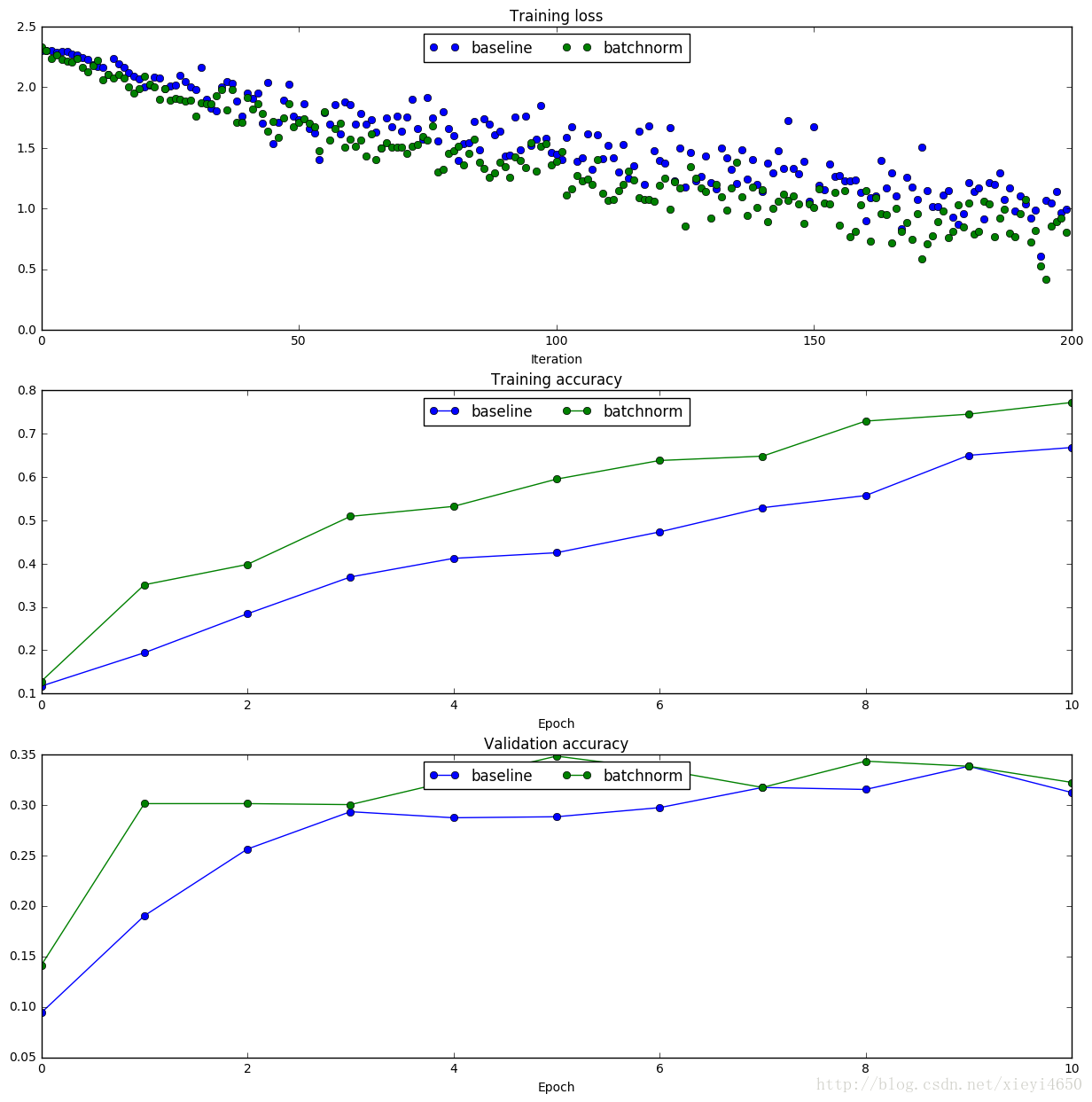

Batch normalization and initialization

We will now run a small experiment to study the interaction of batch normalization and weight initialization.

The first cell will train 8-layer networks both with and without batch normalization using different scales for weight initialization. The second layer will plot training accuracy, validation set accuracy, and training loss as a function of the weight initialization scale.

# Try training a very deep net with batchnorm
hidden_dims = [50, 50, 50, 50, 50, 50, 50]

num_train = 1000
small_data = {
  'X_train': data['X_train'][:num_train],
  'y_train': data['y_train'][:num_train],
  'X_val': data['X_val'],
  'y_val': data['y_val'],
}

bn_solvers = {}
solvers = {}
weight_scales = np.logspace(-4, 0, num=20)
for i, weight_scale in enumerate(weight_scales):
  print 'Running weight scale %d / %d' % (i + 1, len(weight_scales))
  bn_model = FullyConnectedNet(hidden_dims, weight_scale=weight_scale, use_batchnorm=True)
  model = FullyConnectedNet(hidden_dims, weight_scale=weight_scale, use_batchnorm=False)

  bn_solver = Solver(bn_model, small_data,
                  num_epochs=10, batch_size=50,
                  update_rule='adam',
                  optim_config={
                    'learning_rate': 1e-3,
                  },
                  verbose=False, print_every=200)
  bn_solver.train()
  bn_solvers[weight_scale] = bn_solver

  solver = Solver(model, small_data,
                  num_epochs=10, batch_size=50,
                  update_rule='adam',
                  optim_config={
                    'learning_rate': 1e-3,
                  },
                  verbose=False, print_every=200)
  solver.train()
  solvers[weight_scale] = solver

Running weight scale 1 / 20
Running weight scale 2 / 20
Running weight scale 3 / 20
Running weight scale 4 / 20
Running weight scale 5 / 20
Running weight scale 6 / 20
Running weight scale 7 / 20
Running weight scale 8 / 20
Running weight scale 9 / 20
Running weight scale 10 / 20
Running weight scale 11 / 20
Running weight scale 12 / 20
Running weight scale 13 / 20
Running weight scale 14 / 20
Running weight scale 15 / 20
Running weight scale 16 / 20


cs231n/layers.py:588: RuntimeWarning: divide by zero encountered in log
  loss = -np.sum(np.log(probs[np.arange(N), y])) / N


Running weight scale 17 / 20
Running weight scale 18 / 20
Running weight scale 19 / 20
Running weight scale 20 / 20

# Plot results of weight scale experiment
best_train_accs, bn_best_train_accs = [], []
best_val_accs, bn_best_val_accs = [], []
final_train_loss, bn_final_train_loss = [], []

for ws in weight_scales:
  best_train_accs.append(max(solvers[ws].train_acc_history))
  bn_best_train_accs.append(max(bn_solvers[ws].train_acc_history))

  best_val_accs.append(max(solvers[ws].val_acc_history))
  bn_best_val_accs.append(max(bn_solvers[ws].val_acc_history))

  final_train_loss.append(np.mean(solvers[ws].loss_history[-100:]))
  bn_final_train_loss.append(np.mean(bn_solvers[ws].loss_history[-100:]))

plt.subplot(3, 1, 1)
plt.title('Best val accuracy vs weight initialization scale')
plt.xlabel('Weight initialization scale')
plt.ylabel('Best val accuracy')
plt.semilogx(weight_scales, best_val_accs, '-o', label='baseline')
plt.semilogx(weight_scales, bn_best_val_accs, '-o', label='batchnorm')
plt.legend(ncol=2, loc='lower right')

plt.subplot(3, 1, 2)
plt.title('Best train accuracy vs weight initialization scale')
plt.xlabel('Weight initialization scale')
plt.ylabel('Best training accuracy')
plt.semilogx(weight_scales, best_train_accs, '-o', label='baseline')
plt.semilogx(weight_scales, bn_best_train_accs, '-o', label='batchnorm')
plt.legend()

plt.subplot(3, 1, 3)
plt.title('Final training loss vs weight initialization scale')
plt.xlabel('Weight initialization scale')
plt.ylabel('Final training loss')
plt.semilogx(weight_scales, final_train_loss, '-o', label='baseline')
plt.semilogx(weight_scales, bn_final_train_loss, '-o', label='batchnorm')
plt.legend()

plt.gcf().set_size_inches(10, 15)
plt.show()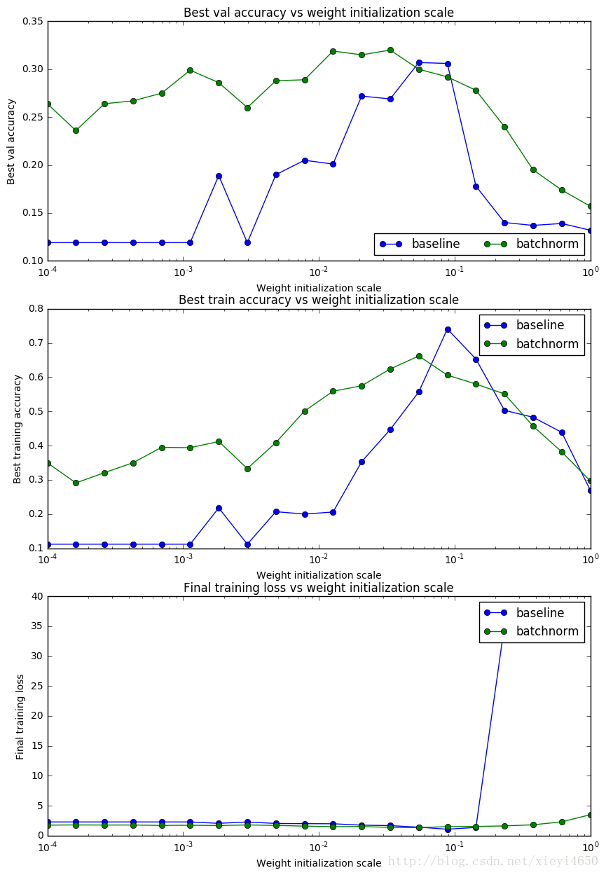

Question:

Describe the results of this experiment, and try to give a reason why the experiment gave the results that it did.

Answer:

过小weight scale很容易会让后面的激活值衰减到0,导致每一层的输出值都一样,capacity能力下降,同理过大的weight scale会使激活值迅速饱和,变为-1和1,所以weight scale必须要选的恰当才能让训练继续下去,从图一可以看到baseline的可训练范围比较小,不适当的weight scale初始化的结果是最终的准确率只比随机猜的准确率高了一点.
Batch normalization人为的将每一层的输出先变为均值为0方差为1的分布,然后再从这个分布缩放和平移到其该有的分布,可以抑制因为初始化不当造成的衰减和饱和.使网络结构不会过于对称,各神经元的输入输出都一样,造成的网络capacity下降.