高斯滤波

前言

高斯滤波器是一种低通滤波器，可以去除低频分量，起到图像平滑的作用。此处高斯是指使用高斯函数作为滤波函数，对卷积模板对应的图像区域进行加权平均。

1. 高斯滤波

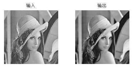
如图所示，原始图像经过高斯模板滑动加权平均之后，便得到模糊过后的输出图像。数学表达为：

也就是说此处存在两个步骤，(1) 高斯模板的生成，(2) 滑窗卷积的实现。

1.1 高斯模板的生成

1.1.1 公式指导

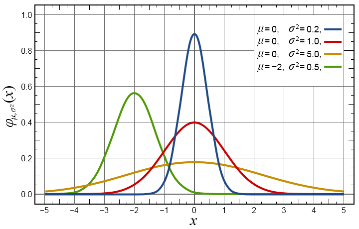
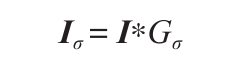
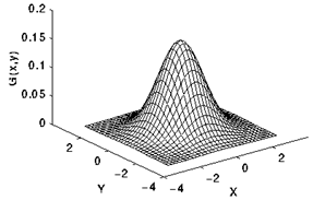
先放一张一维高斯函数的图示，可以看出，sigma越大，则高斯曲线越胖，周围值对中心影响越大，图像越模糊；sigma越小，高斯曲线越精瘦，受周围值影响越小。下面是二维高斯模板的理论指导和图示：

1.1.2 python opencv 生成二维高斯模板

opencv中，当摸板尺寸小于等于7且sigma<=0时候会使用内置（事先计算好的）的模板。

import cv2
import numpy as np

def gaussian_kernel_2d_opencv(kernel_size=3, sigma=0):
    kx = cv2.getGaussianKernel(kernel_size, sigma)
    ky = cv2.getGaussianKernel(kernel_size, sigma)  
    # 如果sigma<=0, sigma = 0.3*((ksize-1)*0.5 - 1) + 0.8
    return np.multiply(kx, np.transpose(ky))

print(gaussian_kernel_2d_opencv(kernel_size=3, sigma=1))
print(gaussian_kernel_2d_opencv(kernel_size=3, sigma=10))
print(gaussian_kernel_2d_opencv(kernel_size=5, sigma=1))

# kernrl_size=3, sigma=1
[[0.07511361 0.1238414  0.07511361]
 [0.1238414  0.20417996 0.1238414 ]
 [0.07511361 0.1238414  0.07511361]]
# kernrl_size=3, sigma=10
[[0.11074074 0.11129583 0.11074074]
 [0.11129583 0.1118537  0.11129583]
 [0.11074074 0.11129583 0.11074074]]
# kernrl_size=5, sigma=1
[[0.00296902 0.01330621 0.02193823 0.01330621 0.00296902]
 [0.01330621 0.0596343  0.09832033 0.0596343  0.01330621]
 [0.02193823 0.09832033 0.16210282 0.09832033 0.02193823]
 [0.01330621 0.0596343  0.09832033 0.0596343  0.01330621]
 [0.00296902 0.01330621 0.02193823 0.01330621 0.00296902]]

1.1.3 python 生成二位高斯模板

import cv2
import numpy as np

def gaussian_2d_kernel(kernel_size=3, sigma=0):
    kernel = np.zeros([kernel_size, kernel_size])
    center = kernel_size // 2
	
	# 确保sigma非负
    if sigma == 0:
        sigma = 0.3 * ((kernel_size - 1) * 0.5 - 1) + 0.8

    s = 2 * (sigma ** 2)
    sum_val = 0
    for i in range(0, kernel_size):
        for j in range(0, kernel_size):
            x = i - center
            y = j - center
            # 此处未计算1/(2*pi*sigma), 其会在最终求和取平均值(归一化)后约掉
            kernel[i, j] = np.exp(-(x ** 2 + y ** 2) / s)
            sum_val += kernel[i, j]
    return kernel / sum_val

print(gaussian_kernel_2d_opencv(kernel_size=3, sigma=1))
print(gaussian_kernel_2d_opencv(kernel_size=3, sigma=10))
print(gaussian_kernel_2d_opencv(kernel_size=5, sigma=1))

# kernrl_size=3, sigma=1
[[0.07511361 0.1238414  0.07511361]
 [0.1238414  0.20417996 0.1238414 ]
 [0.07511361 0.1238414  0.07511361]]
# kernrl_size=3, sigma=10
[[0.11074074 0.11129583 0.11074074]
 [0.11129583 0.1118537  0.11129583]
 [0.11074074 0.11129583 0.11074074]]
# kernrl_size=5, sigma=1
[[0.00296902 0.01330621 0.02193823 0.01330621 0.00296902]
 [0.01330621 0.0596343  0.09832033 0.0596343  0.01330621]
 [0.02193823 0.09832033 0.16210282 0.09832033 0.02193823]
 [0.01330621 0.0596343  0.09832033 0.0596343  0.01330621]
 [0.00296902 0.01330621 0.02193823 0.01330621 0.00296902]]

1.2 滑窗卷积

1.2.1 python opencv 卷积

import cv2
import numpy as np
import matplotlib.pyplot as plt

def gaussian_kernel_2d_opencv(kernel_size=3, sigma=1):
    kx = cv2.getGaussianKernel(kernel_size, sigma)
    ky = cv2.getGaussianKernel(kernel_size, sigma)
    return np.multiply(kx, np.transpose(ky))

image = cv2.imread('lena512.bmp'， 0)

# two step: getGaussianKernel & filter2D
kernel3_1 = gaussian_kernel_2d_opencv(kernel_size=3, sigma=1)
dst3_1 = cv2.filter2D(image, -1, kernel3_1)

kernel3_10 = gaussian_kernel_2d_opencv(kernel_size=3, sigma=10)
dst3_10 = cv2.filter2D(image, -1, kernel3_10)

kernel5_1 = gaussian_kernel_2d_opencv(kernel_size=5, sigma=1)
dst5_1 = cv2.filter2D(image, -1, kernel5_1)

# one step: GaussianBlur
DST3_1 = cv2.GaussianBlur(image, ksize=(3, 3), sigmaX=1)
DST3_10 = cv2.GaussianBlur(image, ksize=(3, 3), sigmaX=10)
DST5_1 = cv2.GaussianBlur(image, ksize=(5, 5), sigmaX=1)

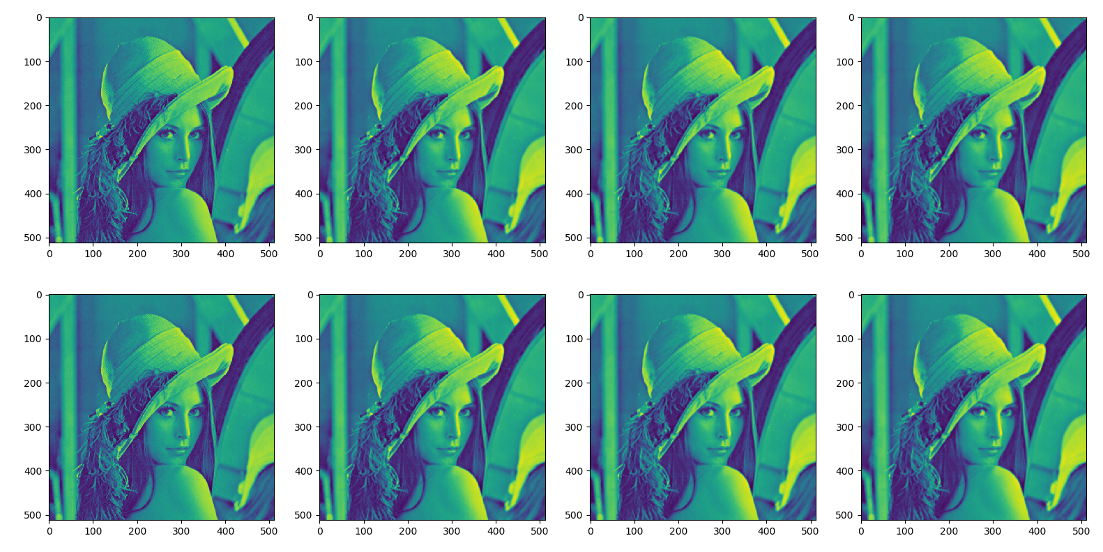
plt.figure()
plt.subplot(241)
plt.imshow(image)
plt.subplot(242)
plt.imshow(dst3_1)
plt.subplot(243)
plt.imshow(dst3_10)
plt.subplot(244)
plt.imshow(dst5_1)
plt.subplot(245)
plt.imshow(image)
plt.subplot(246)
plt.imshow(DST3_1)
plt.subplot(247)
plt.imshow(DST3_10)
plt.subplot(248)
plt.imshow(DST5_1)
plt.show()

1.2.2 python 自己写卷积

import numpy as np
import cv2
import matplotlib.pyplot as plt

# 获取卷积核
def gaussian_kernel_2d_opencv(kernel_size=3, sigma=1):
    kx = cv2.getGaussianKernel(kernel_size, sigma)
    ky = cv2.getGaussianKernel(kernel_size, sigma)
    return np.multiply(kx, np.transpose(ky))

# 定义卷积操作的函数
def conv(image, kernel):
    height, width = image.shape
    kernel_row, kernel_col = kernel.shape

    # 经滑动卷积操作后得到的新的图像的尺寸
    new_h = height - kernel_row + 1
    new_w = width - kernel_col + 1
    new_image = np.zeros((new_h, new_w), dtype=np.float)

    # 进行卷积操作,实则是对应的窗口覆盖下的矩阵对应元素值相乘,卷积操作
    for i in range(new_w):
        for j in range(new_h):
            new_image[i, j] = np.sum(image[i:i+kernel_row, j:j+kernel_col] * kernel)

    # 去掉矩阵乘法后的小于0的和大于255的原值,重置为0和255
    new_image = new_image.clip(0, 255)
    new_image = np.rint(new_image).astype('uint8')
    return new_image

image = cv2.imread('lena512.bmp', flags=0)
print(image.shape)

# two step: getGaussianKernel & conv
kernel3_1 = gaussian_kernel_2d_opencv(kernel_size=3, sigma=1)
dst3_1 = conv(image, kernel3_1)

kernel3_10 = gaussian_kernel_2d_opencv(kernel_size=3, sigma=10)
dst3_10 = conv(image, kernel3_10)

kernel5_1 = gaussian_kernel_2d_opencv(kernel_size=5, sigma=1)
dst5_1 = conv(image, kernel5_1)

# one step: GaussianBlur
DST3_1 = cv2.GaussianBlur(image, ksize=(3, 3), sigmaX=1)
DST3_10 = cv2.GaussianBlur(image, ksize=(3, 3), sigmaX=10)
DST5_1 = cv2.GaussianBlur(image, ksize=(5, 5), sigmaX=1)

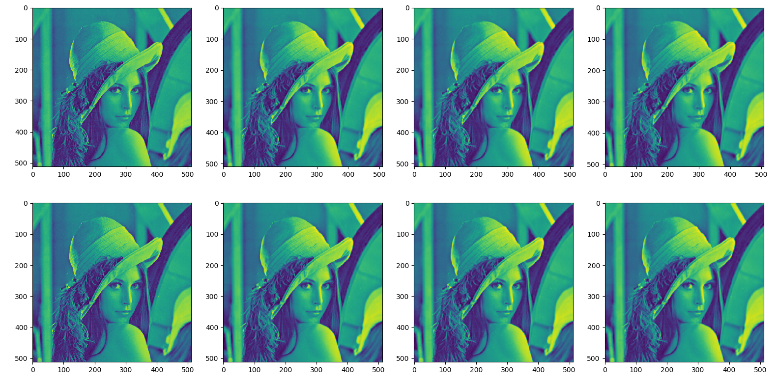
plt.figure()
plt.subplot(241)
plt.imshow(image)
plt.subplot(242)
plt.imshow(dst3_1)
plt.subplot(243)
plt.imshow(dst3_10)
plt.subplot(244)
plt.imshow(dst5_1)
plt.subplot(245)
plt.imshow(image)
plt.subplot(246)
plt.imshow(DST3_1)
plt.subplot(247)
plt.imshow(DST3_10)
plt.subplot(248)
plt.imshow(DST5_1)
plt.show()

1.3 傅里叶变换卷积

学过图像处理或者信号处理的同学应该都听说过时域卷积=频域相乘，当然这背后有严谨的数学推导证明，才疏学浅，此处不做证明。

假设输入图像的大小为len=hw，卷积核大小k_len＝mn；通常len>>k_len。其主要步骤如下：

• 对输入图像A做傅里叶变换；
• 对卷积核B做傅里叶变换，但是由于卷积核与输入图像尺寸不一样，需要将卷积核扩展，即将卷积核倒置后，补len-k_len个０；
• 将A、B傅里叶变换的结果相乘，即对应位相乘获得结果C；
• 对C做傅里叶逆变换，得到结果D，在D中每隔k_len的值实部取出来，就是图像卷积的结果。因为图像卷积其实就是对应位相乘，所以需要每隔k_len取值；

1.3.1 python numpy & opencv 傅里叶变换

import cv2
import numpy as np
from matplotlib import pyplot as plt

# read image
img = cv2.imread('lena512.bmp', 0)

# ------------------------- numpy ------------------------- #
# opencv的频域结果的复数是以(512， 512)，每个数字都是一个虚数
# 1. fft:将空间域转化为频率域
fft = np.fft.fft2(img)
# 2. fftshift:将低频部分移动到图像中心(复数)
fft_shift = np.fft.fftshift(fft)
# 3. ifftshift: 将低频部分从中心移动回到左上角（复数）
ifft_shift = np.fft.ifftshift(fft_shift)
# 4. ifft2:将频率域转化回空间域（复数）
ifft = np.fft.ifft2(ifft_shift)

# ------------- magnitude_spectrum ---------------#
# 目的：先求复数的模，进而进行归一化
magnitude_of_fft = 20 * np.log(np.abs(fft))
magnitude_of_fft_shift = 20 * np.log(np.abs(fft_shift))
magnitude_of_ifft_shift = 20 * np.log(np.abs(ifft_shift))
magnitude_of_ifft = np.abs(ifft)


# ------------------------------ opencv -------------------- #
# opencv的频域结果的复数是以(512， 512， 2)，第一层代表实部，第二层代表虚部
dft = cv2.dft(np.float32(img), flags=cv2.DFT_COMPLEX_OUTPUT)
dft_shift = np.fft.fftshift(dft)
idft_shift = np.fft.ifftshift(dft_shift)
idft = cv2.idft(idft_shift)

# ------------- magnitude_spectrum ---------------#
# 目的：先求复数的模，进而进行归一化
magnitude_of_dft = 20 * np.log(cv2.magnitude(dft[:, :, 0], dft[:, :, 1]))
magnitude_of_dft_shift = 20 * np.log(cv2.magnitude(dft_shift[:, :, 0], dft_shift[:, :, 1]))
magnitude_of_idft_shift = 20 * np.log(cv2.magnitude(idft_shift[:, :, 0], idft_shift[:, :, 1]))
magnitude_of_idft = cv2.magnitude(idft[:, :, 0], idft[:, :, 1])


plt.subplot(2, 5, 1)
plt.title('original Image')
plt.imshow(img, cmap='gray')
plt.subplot(2, 5, 2)
plt.title('magnitude of fft')
plt.imshow(magnitude_of_fft, cmap='gray')
plt.subplot(2, 5, 3)
plt.title('magnitude of fft_shift')
plt.imshow(magnitude_of_fft_shift, cmap='gray')
plt.subplot(2, 5, 4)
plt.title('magnitude of ifft_shift')
plt.imshow(magnitude_of_ifft_shift, cmap='gray')
plt.subplot(2, 5, 5)
plt.title('magnitude of ifft')
plt.imshow(magnitude_of_ifft, cmap='gray')

plt.subplot(2, 5, 6)
plt.title('original Image')
plt.imshow(img, cmap='gray')
plt.subplot(2, 5, 7)
plt.title('magnitude of dft')
plt.imshow(magnitude_of_dft, cmap='gray')
plt.subplot(2, 5, 8)
plt.title('magnitude of dft_shift')
plt.imshow(magnitude_of_dft_shift, cmap='gray')
plt.subplot(2, 5, 9)
plt.title('magnitude of dft_shift')
plt.imshow(magnitude_of_dft_shift, cmap='gray')
plt.subplot(2, 5, 10)
plt.title('magnitude of idft')
plt.imshow(magnitude_of_idft, cmap='gray')
plt.show()

[外链图片转存失败,源站可能有防盗链机制,建议将图片保存下来直接上传(img-SEk2xzu9-1607922626194)(https://cdn.jsdelivr.net/gh/niecongchong/csdn_img@master/img/2019-08-06-9.png)]

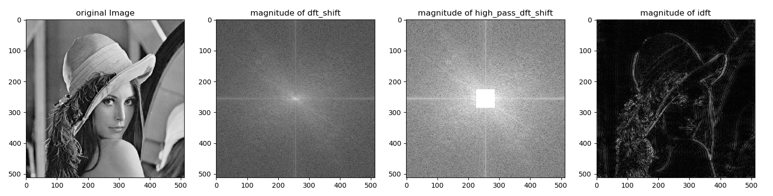
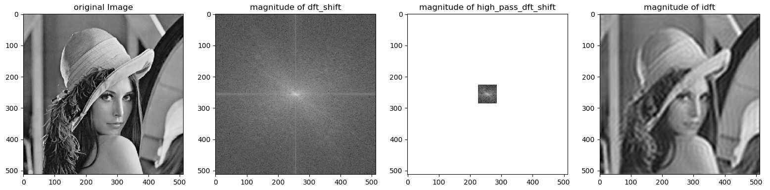
1.3.2 python 傅里叶变换 & 高通滤波

import cv2
import numpy as np
from matplotlib import pyplot as plt

# read image
img = cv2.imread('lena512.bmp', 0)

# 傅里叶正变换
dft = cv2.dft(np.float32(img), flags=cv2.DFT_COMPLEX_OUTPUT)
dft_shift = np.fft.fftshift(dft)

# 高通滤波
high_pass_dft_shift = dft_shift.copy()
rows, cols = img.shape
crow, ccol = int(rows/2), int(cols/2)
high_pass_dft_shift[crow - 30: crow + 30, ccol - 30: ccol + 30] = 0

# 傅里叶逆变换
idft_shift = np.fft.ifftshift(high_pass_dft_shift)
idft = cv2.idft(idft_shift)

# ------------- magnitude_spectrum ---------------#
# 目的：先求复数的模，进而进行归一化
magnitude_of_dft_shift = 20 * np.log(cv2.magnitude(dft_shift[:, :, 0], dft_shift[:, :, 1]))
magnitude_of_high_pass_dft_shift = 20 * np.log(cv2.magnitude(high_pass_dft_shift[:, :, 0], high_pass_dft_shift[:, :, 1]))
magnitude_of_idft = cv2.magnitude(idft[:, :, 0], idft[:, :, 1])

plt.subplot(141)
plt.title('original Image')
plt.imshow(img, cmap='gray')
plt.subplot(142)
plt.title('magnitude of dft_shift')
plt.imshow(magnitude_of_dft_shift, cmap='gray')
plt.subplot(143)
plt.title('magnitude of high_pass_dft_shift')
plt.imshow(magnitude_of_high_pass_dft_shift, cmap='gray')
plt.subplot(144)
plt.title('magnitude of idft')
plt.imshow(magnitude_of_idft, cmap='gray')
plt.show()

1.3.3 python 傅里叶变换 & 低通滤波

import cv2
import numpy as np
from matplotlib import pyplot as plt

# read image
img = cv2.imread('lena512.bmp', 0)

# 傅里叶正变换
dft = cv2.dft(np.float32(img), flags=cv2.DFT_COMPLEX_OUTPUT)
dft_shift = np.fft.fftshift(dft)

# 低通滤波: 创建一个掩码，中心为1，其余为0
rows, cols = img.shape
crow, ccol = int(rows/2), int(cols/2)
mask = np.zeros((rows, cols, 2), np.uint8)
mask[crow - 30: crow + 30, ccol - 30: ccol + 30] = 1

low_pass_dft_shift = dft_shift * mask

# 傅里叶逆变换
idft_shift = np.fft.ifftshift(low_pass_dft_shift)
idft = cv2.idft(idft_shift)

# ------------- magnitude_spectrum ---------------#
# 目的：先求复数的模，进而进行归一化
magnitude_of_dft_shift = 20 * np.log(cv2.magnitude(dft_shift[:, :, 0], dft_shift[:, :, 1]))
magnitude_of_low_pass_dft_shift = 20 * np.log(cv2.magnitude(low_pass_dft_shift[:, :, 0], low_pass_dft_shift[:, :, 1]))
magnitude_of_idft = cv2.magnitude(idft[:, :, 0], idft[:, :, 1])


plt.subplot(141)
plt.title('original Image')
plt.imshow(img, cmap='gray')
plt.subplot(142)
plt.title('magnitude of dft_shift')
plt.imshow(magnitude_of_dft_shift, cmap='gray')
plt.subplot(143)
plt.title('magnitude of low_pass_dft_shift')
plt.imshow(magnitude_of_low_pass_dft_shift, cmap='gray')
plt.subplot(144)
plt.title('magnitude of idft')
plt.imshow(magnitude_of_idft, cmap='gray')
plt.show()

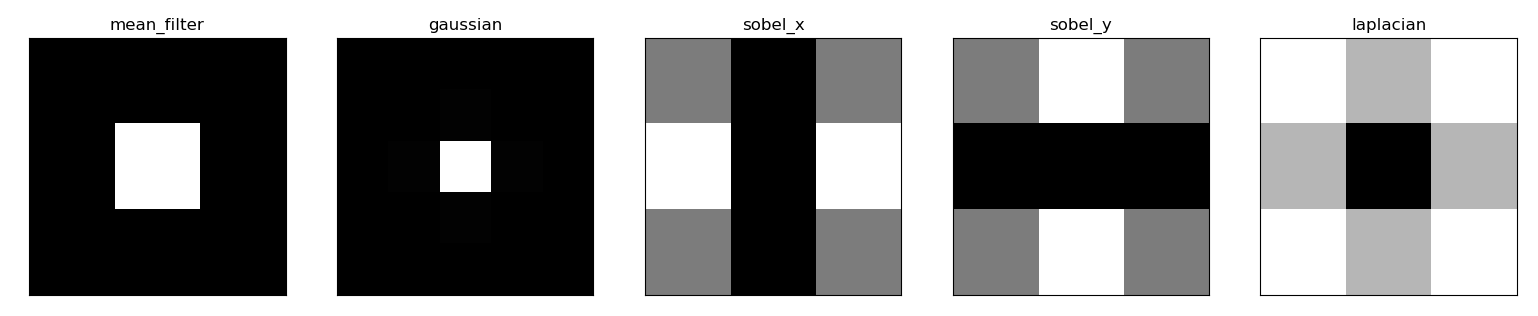
1.3.4 python 卷积核的傅里叶变换

import cv2 as cv
import numpy as np
from matplotlib import pyplot as plt

# 平均滤波器
mean_filter = np.ones((3, 3))

# 高斯滤波器
x = cv.getGaussianKernel(5, 10)
gaussian = x * x.T

# 不同的边缘检测滤波器
# sobel in x direction
sobel_x = np.array([[-1, 0, 1],
                    [-2, 0, 2],
                    [-1, 0, 1]])

# sobel in y direction
sobel_y = np.array([[-1, -2, -1],
                    [ 0,  0,  0],
                    [ 1,  2,  1]])

# laplacian
laplacian = np.array([[0,  1, 0],
                     [1, -4, 1],
                     [0,  1, 0]])

filters = [mean_filter, gaussian, sobel_x, sobel_y, laplacian]
filter_name = ['mean_filter', 'gaussian', 'sobel_x', 'sobel_y', 'laplacian']
fft_filters = [np.fft.fft2(x) for x in filters]
fft_shift = [np.fft.fftshift(y) for y in fft_filters]
mag_spectrum = [np.log(np.abs(z)+1) for z in fft_shift]

for i in range(5):
    plt.subplot(1, 5, i+1), plt.imshow(mag_spectrum[i], cmap='gray')
    plt.title(filter_name[i]), plt.xticks([]), plt.yticks([])

plt.show()

1.3.5 python 傅里叶变换执行卷积操作

卷积定理表明，时域中的循环卷积相当于频域的点积。通常，这种方法需要卷积核的尺寸大小接近输入图像的尺寸。具体运算时，需要将输入图像和卷积核变换到频率域中的相同的大小，进而对两者执行频域乘法，最后进行傅里叶逆变换，要得到与原始图像相同尺寸的处理后的图像，需要进行图像裁剪。

import cv2
import numpy as np
from matplotlib import pyplot as plt
from scipy import signal

# read image
img = cv2.imread('lena512.bmp', 0)

# general gaussian kernel
x = cv2.getGaussianKernel(21, 10)
gaussian = x * x.T

# 傅里叶正变换，先计算频域中两者的尺寸
img_row, img_col = img.shape
kernel_row, kernel_col = gaussian.shape
size_row = img_row + kernel_row - 1
size_col = img_col + kernel_col - 1
out_row = 2 ** (int(np.log2(size_row)) + 1)
out_col = 2 ** (int(np.log2(size_col)) + 1)

fft = np.fft.fft2(img, (out_row, out_col))
fft_shift = np.fft.fftshift(fft)

fft_gaussian = np.fft.fft2(gaussian, (out_row, out_col))
fft_gaussian_shift = np.fft.fftshift(fft_gaussian)

# 频域乘法：掩模
fft_shift_mask = fft_shift * fft_gaussian_shift

# 傅里叶逆变换
ifft_shift = np.fft.ifftshift(fft_shift_mask)
ifft = np.fft.ifft2(ifft_shift)

# ------------- magnitude_spectrum ---------------#
# 目的：先求复数的模，进而进行归一化
magnitude_of_fft_shift = 20 * np.log(np.abs(fft_shift))
magnitude_of_fft_gaussian_shift = np.log(np.abs(fft_gaussian_shift)) + 1
magnitude_of_fft_shift_mask = 20 * np.log(np.abs(fft_shift_mask))
# 裁剪（先把图像区域裁出来，再对图像区域进行中心裁剪，去除边缘填充的像素）
magnitude_of_ifft = ifft.real[0: size_row, 0: size_col]
row, col = magnitude_of_ifft.shape
magnitude_of_ifft = magnitude_of_ifft[row // 2 - img_row // 2: row // 2 - img_row // 2 + img_row,
                                      col // 2 - img_col // 2: col // 2 - img_col // 2 + img_col]

plt.subplot(151)
plt.title('original Image')
plt.imshow(img, cmap='gray')
plt.subplot(152)
plt.title('magnitude of fft_shift')
plt.imshow(magnitude_of_fft_shift, cmap='gray')
plt.subplot(153)
plt.title('magnitude of fft_gaussian_shift')
plt.imshow(magnitude_of_fft_gaussian_shift, cmap='gray')
plt.subplot(154)
plt.title('magnitude of fft_shift_mask')
plt.imshow(magnitude_of_fft_shift_mask, cmap='gray')
plt.subplot(155)
plt.title('magnitude of ifft')
plt.imshow(magnitude_of_ifft, cmap='gray')
plt.show()