《动手学深度学习》（二）-- 多层感知机

长路漫漫2021

已于 2022-07-01 11:01:47 修改

阅读量1.2k

点赞数

分类专栏： # Deep Learning 文章标签：深度学习 pytorch 人工智能多层感知机动手学深度学习

于 2022-07-01 11:01:27 首次发布

本文链接：https://blog.csdn.net/xq151750111/article/details/125554605

版权

Deep Learning 专栏收录该内容

13 篇文章 16 订阅

订阅专栏

1 多层感知机

1.1 从零开始实现

本节将继续使⽤Fashion-MNIST图像分类数据集，数据导入步骤和上一节一样，本节将不再展示。

import torch
from d2l import torch as d2l
import torch.nn.functional as F
from torch.utils.data import DataLoader
from torch.utils import data
from torchvision import transforms
from torch import nn

mnist_train = FashionMnistDataset("../dataset/fashion-mnist", "train-images-idx3-ubyte.gz", "train-labels-idx1-ubyte.gz", transform=transforms.ToTensor())
mnist_test = FashionMnistDataset("../dataset/fashion-mnist", "t10k-images-idx3-ubyte.gz", "t10k-labels-idx1-ubyte.gz", transform=transforms.ToTensor())
train_loader = DataLoader(mnist_train, batch_size=256, shuffle=True, num_workers=4)
test_loader = DataLoader(mnist_test, batch_size=256, shuffle=False, num_workers=4)

1. 初始化模型参数

⾸先，我们将实现⼀个具有单隐藏层的多层感知机，它包含256个隐藏单元。注意，我们可以将这两个变量都视为超参数。通常，我们选择2的若⼲次幂作为层的宽度。因为内存在硬件中的分配和寻址⽅式，这么做往往可以在计算上更⾼效。

⽤⼏个张量来表⽰我们的参数。注意，对于每⼀层我们都要记录⼀个权重矩阵和⼀个偏置向量。跟以前⼀样，我们要为这些参数的损失的梯度分配内存。

num_inputs, num_outputs, num_hiddens = 784, 10, 256
W1 = nn.Parameter(torch.randn(num_inputs, num_hiddens, requires_grad=True) * 0.01)
b1 = nn.Parameter(torch.zeros(num_hiddens, requires_grad=True))
W2 = nn.Parameter(torch.randn(num_hiddens, num_outputs, requires_grad=True) * 0.01)
b2 = nn.Parameter(torch.zeros(num_outputs, requires_grad=True))
params = [W1, b1, W2, b2]

2. 激活函数

def relu(X):
    a = torch.zeros_like(X)
    return torch.max(X, a)

3. 模型
使⽤reshape将每个⼆维图像转换为⼀个⻓度为num_inputs的向量。

def net(X):
    X = X.reshape((-1, num_inputs))
    H = relu(X@W1 + b1)
    return (H@W2 + b2)

4. 损失函数

loss = nn.CrossEntropyLoss()

5. 训练

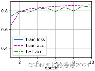
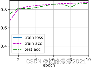
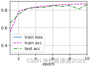
多层感知机的训练过程与softmax回归的训练过程完全相同。可以直接调⽤d2l包的train_ch3函数，将迭代周期数设置为10，并将学习率设置为0.1。

num_epoches, lr = 10, 0.1
optimizer = torch.optim.SGD(params, lr=lr)
d2l.train_ch3(net, train_loader, test_loader, loss, num_epoches, optimizer)

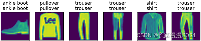
6. 评估模型

d2l.predict_ch3(net, test_loader)

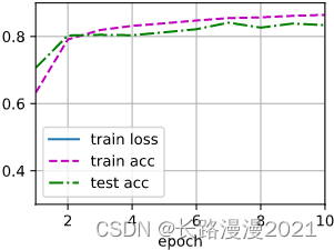
1.2 简洁实现

这里和上一节的softmax回归的简洁实现相比，唯一的区别是这里使用了2个全连接层，第一层是隐藏层，包含256个隐藏单元，并使用ReLU激活函数。

net = nn.Sequential(nn.Flatten(), nn.Linear(784, 256), nn.ReLU(), nn.Linear(256, 10))
def init_weights(m):
    if isinstance(m, nn.Linear):
        nn.init.normal_(m.weight, std=0.01)

net.apply(init_weights)

lr, num_epoches = 0.1, 10
loss = nn.CrossEntropyLoss()
optimizer = torch.optim.SGD(net.parameters(), lr=lr)
d2l.train_ch3(net, train_loader, test_loader, loss, num_epoches, optimizer)

2 多项式回归

本节主要以不同阶数的多项式进行回归实验，从而体会过拟合和欠拟合。

import torch
import numpy as np
import torch
from torch import nn
from d2l import torch as d2l
import math

1. 生成数据集
给定 $x$ ，使用以下三阶多项式来⽣成训练和测试数据的标签：
$\frac{x^{2}}{2 !}+5.6 \frac{x^{3}}{3 !}+\epsilon \text { where } \epsilon \sim \mathcal{N}\left(0,0.1^{2}\right)$

噪声 $\epsilon$ 项服从均值为0且标准差为0.1的正态分布。在优化的过程中，我们通常希望避免⾮常⼤的梯度值或损失值。这就是我们将特征从 $x^i$ 调整为 $\frac{x^i}{i!}$ 的原因，这样可以避免很⼤的i带来的特别⼤的指数值。为训练集和测试集各⽣成100个样本。

max_degree = 20                 # 多项式回归的最大阶数
n_train, n_test = 100, 100      # 训练集和测试接大小
true_w = np.zeros(max_degree)   # 分配大量的空间
true_w[0:4] = np.array([5, 1.2, -3.4, 5.6])

features = np.random.normal(size=(n_train + n_test, 1))
np.random.shuffle(features)
poly_features = np.power(features, np.arange(max_degree).reshape(1, -1))        # 200 * 20 特征矩阵
for i in range(max_degree):
    poly_features[:, i] /= math.gamma(i+1)      # gamma(n) = (n-1)!
    # labels的维度：(n_train+n_test, )
labels = np.dot(poly_features, true_w)
labels += np.random.normal(scale=0.1, size=labels.shape)        # 加上误差

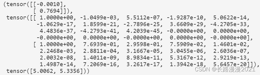
同样，存储在poly_features中的单项式由gamma函数重新缩放，其中 $\Gamma(n)=(n-1)!$ 。从⽣成的数据集中查看⼀下前2个样本，第⼀个值是与偏置相对应的常量特征。

# NumPyndarray转换为tensor
true_w, features, poly_features, labels = [torch.tensor(x, dtype=torch.float32) for x in [true_w, features, poly_features, labels]]
features[:2], poly_features[:2, :], labels[:2]

2. 训练和测试

⾸先实现⼀个函数来评估模型在给定数据集上的损失。

def evaluate_loss(net, data_loader, loss):
    """评估给定数据集上模型的损失"""
    metric = d2l.Accumulator(2)     # 损失的总和，样本数量
    for X, y in data_loader:
        out = net(X)
        y = y.reshape(out.shape)
        l = loss(out, y)
        metric.add(l.sum(), l.numel())
    return metric[0] / metric[1]

3. 定义训练函数

def train(train_features, test_features, train_labels, test_labels, num_epoches=400):
    loss = nn.MSELoss(reduction='none')
    input_shape = train_features.shape[-1]
    # 不设置偏置，因为已经在多项式特征中实现了它
    net = nn.Sequential(nn.Linear(input_shape, 1, bias=False))
    batch_size = min(10, train_labels.shape[0])
    train_iter = d2l.load_array((train_features, train_labels.reshape(-1, 1)), batch_size)
    test_iter = d2l.load_array((test_features, test_labels.reshape(-1, 1)), batch_size, is_train=False)
    trainer = torch.optim.SGD(net.parameters(), lr=0.001)
    animator = d2l.Animator(xlabel='epoch', ylabel='loss', yscale='log', xlim=[1, num_epoches], ylim=[1e-3, 1e2], legend=['train', 'test'])
    for epoch in range(num_epoches):
        d2l.train_epoch_ch3(net, train_iter, loss, trainer)
        if epoch == 0 or (epoch+1) % 20 == 0:
            animator.add(epoch+1, (evaluate_loss(net, train_iter, loss), (evaluate_loss(net, test_iter, loss))))
    print('weight:', net[0].weight.data.numpy())

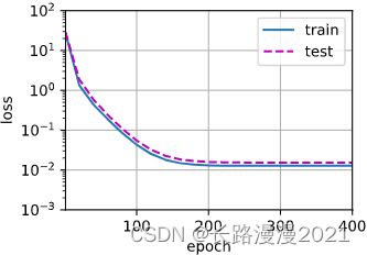
使⽤三阶多项式函数，它与数据⽣成函数的阶数相同。结果表明，该模型能有效降低训练损失和测试损失。学习到的模型参数也接近真实值 $w = [5, 1.2, - 3.4, 5.6]$ 。

# 从多项式特征中选择前4个维度，即1,x,x^2/2!,x^3/3!
train(poly_features[:n_train, :4], poly_features[n_train:, :4], labels[:n_train], labels[n_train:])

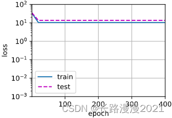
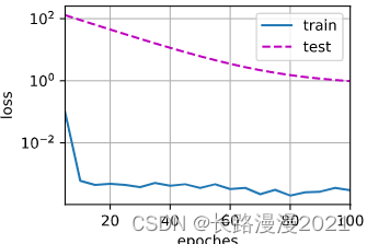
再看看线性函数拟合，减少该模型的训练损失相对困难。在最后⼀个迭代周期完成后，训练损失仍然很⾼。当⽤来拟合⾮线性模式（如这⾥的三阶多项式函数）时，线性模型容易⽋拟合。

# 从多项式特征中选择前2个维度，即1,x
train(poly_features[:n_train, :2], poly_features[n_train:, :2], labels[:n_train], labels[n_train:])

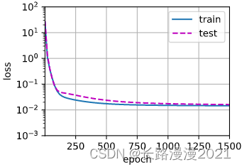
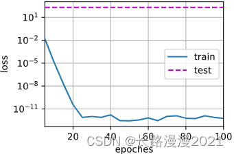
尝试使⽤⼀个阶数过⾼的多项式来训练模型。在这种情况下，没有⾜够的数据⽤于学到⾼阶系数应该具有接近于零的值。因此，这个过于复杂的模型会轻易受到训练数据中噪声的影响。虽然训练损失可以有效地降低，但测试损失仍然很⾼。结果表明，复杂模型对数据造成了过拟合。

# 从多项式特征中选择所有维度
train(poly_features[:n_train, :], poly_features[n_train:, :], labels[:n_train], labels[n_train:], num_epoches=1500)

3 权重衰减

3.1 高维线性回归

这里的权重衰减也就是对权重加上惩罚项，这里以线性回归为例。

import torch
from torch import nn
from d2l import torch as d2l

1. 生成数据

生成公式如下：
$y=0.05+\sum_{i=1}^{d} 0.01 x_{i}+\epsilon \text { where } \epsilon \sim \mathcal{N}\left(0,0.01^{2}\right)$

选择标签是关于输⼊的线性函数。标签同时被均值为0，标准差为0.01⾼斯噪声破坏。为了使过拟合的效果更加明显，我们可以将问题的维数增加到d = 200，并使⽤⼀个只包含20个样本的小训练集。

n_train, n_test, num_inputs, batch_size = 20, 100, 200, 5
true_w, true_b = torch.ones((num_inputs, 1)) * 0.01, 0.05
train_data = d2l.synthetic_data(true_w, true_b, n_train)
train_iter = d2l.load_array(train_data, batch_size)
test_data = d2l.synthetic_data(true_w, true_b, n_test)
test_iter = d2l.load_array(test_data, batch_size, is_train=False)

2. 初始化模型参数

定义⼀个函数来随机初始化模型参数。

def init_params():
    w = torch.normal(0, 1, size=(num_inputs, 1), requires_grad=True)
    b = torch.zeros(1, requires_grad=True)
    return [w, b]

3. 定义L2惩罚项

实现这⼀惩罚最⽅便的⽅法是对所有项求平⽅后并将它们求和。

def l2_penalty(w):
    return torch.sum(w.pow(2)) / 2

4. 训练

def train(lambd):
    w, b = init_params()
    net, loss = lambda X: d2l.linreg(X, w, b), d2l.squared_loss
    num_epoches, lr = 100, 0.003
    animator = d2l.Animator(xlabel='epoches', ylabel='loss', yscale='log', xlim=[5, num_epoches], legend=['train', 'test'])
    for epoch in range(num_epoches):
        for X, y in train_iter:
            # 增加了L2范数惩罚项，
            # ⼴播机制使l2_penalty(w)成为⼀个⻓度为batch_size的向量
            l = loss(net(X), y) + lambd * l2_penalty(w)
            l.sum().backward()
            d2l.sgd([w, b], lr, batch_size)
            if (epoch+1) % 5 == 0:
                animator.add(epoch+1, (d2l.evaluate_loss(net, train_iter, loss), d2l.evaluate_loss(net, test_iter, loss)))
        print('w的L2范数是：', torch.norm(w).item())

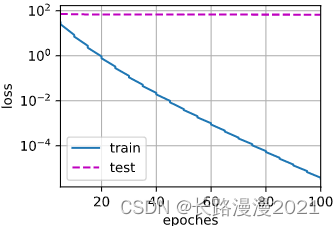
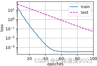
我们现在⽤lambd = 0禁⽤权重衰减后运⾏这个代码。注意，这⾥训练误差在减少，但测试误差没有减少，这意味着出现了严重的过拟合。

train(lambd=0)

我们使⽤权重衰减来运⾏代码。注意，在这⾥训练误差增⼤，但测试误差减小。这正是我们期望从正则化中得到的效果。

train(lambd=3)

由于权重衰减在神经⽹络优化中很常⽤，深度学习框架为了便于我们使⽤权重衰减，将权重衰减集成到优化算法中，以便与任何损失函数结合使⽤。此外，这种集成还有计算上的好处，允许在不增加任何额外的计算开销的情况下向算法中添加权重衰减。由于更新的权重衰减部分仅依赖于每个参数的当前值，因此优化器必须⾄少接触每个参数⼀次。

在下⾯的代码中，我们在实例化优化器时直接通过weight_decay指定weight decay超参数。默认情况下，PyTorch同时衰减权重和偏移。这⾥我们只为权重设置了weight_decay，所以偏置参数b不会衰减。

def train_concise(wd):
    net = nn.Sequential(nn.Linear(num_inputs, 1))
    for param in net.parameters():
        param.data.normal_()
    loss = nn.MSELoss(reduction='none')
    num_epoches, lr = 100, 0.003
    # 偏置参数没有衰减
    trainer = torch.optim.SGD([{'params': net[0].weight, 'weight_decay': wd}, {"params": net[0].bias
    }], lr = lr)
    animator = d2l.Animator(xlabel='epoches', ylabel='loss', yscale='log', xlim=[5, num_epoches], legend=['train', 'test'])
    for epoch in range(num_epoches):
        for X, y in train_iter:
            trainer.zero_grad()
            l = loss(net(X), y)
            l.sum().backward()
            trainer.step()
        if (epoch+1) % 5 == 0:
            animator.add(epoch+1, (d2l.evaluate_loss(net, train_iter, loss), d2l.evaluate_loss(net, test_iter, loss)))

    print('w的L2范数：', net[0].weight.norm().item())

train_concise(0)

train_concise(3)

4 暂退法

4.1 从零开始实现

在标准暂退法正则化中，通过按保留（未丢弃）的节点的分数进⾏规范化来消除每⼀层的偏差。换⾔之，每个中间活性值 $h$ 以暂退概率 $p$ 由随机变量 $h^{'}$ 替换，如下所⽰：
$h^{\prime}= \begin{cases}0 & \text { 概率为 } p \\ \frac{h}{1-p} & \text { 其他情况 }\end{cases}$
根据此模型的设计，其期望值保值不变，即 $E [h^{'}] = h$ 。

要实现单层的暂退法函数，我们从均匀分布U[0, 1]中抽取样本，样本数与这层神经⽹络的维度⼀致。然后保留那些对应样本⼤于p的节点，把剩下的丢弃。

实现dropout_layer函数，该函数以dropout的概率丢弃张量输⼊X中的元素，如上所述重新缩放剩余部分：将剩余部分除以1.0-dropout。

1. 随机失活

import torch 
from torch import nn
from d2l import torch as d2l

def dropout_layer(X, dropout):
    assert 0 <= dropout <= 1
    # 在本情况，所有元素都被抛弃
    if dropout == 1:
        return torch.zeros_like(X)
    # 在本情况中，所有元素都被保留
    if dropout == 0:
        return X
    mask = (torch.rand(X.shape) > dropout).float()
    return mask * X / (1.0 - dropout)

2. 定义模型

定义具有两个隐藏层的多层感知机，每个隐藏层包含256个单元。将暂退法应⽤于每个隐藏层的输出（在激活函数之后），并且可以为每⼀层分别设置暂退概率：常⻅的技巧是在靠近输⼊层的地⽅设置较低的暂退概率。下⾯的模型将第⼀个和第⼆个隐藏层的暂退概率分别设置为0.2和0.5，并且暂退法只在训练期间有效。

num_inputs, num_outputs, num_hiddens1, num_hiddens2 = 784, 10, 256, 256
dropout1, dropout2 = 0.2, 0.5
class Net(nn.Module):
    def __init__(self, num_inputs, num_outputs, num_hiddens, num_hiddens2, is_training=True):
        super(Net, self).__init__()
        self.num_inputs = num_inputs
        self.training = is_training
        self.lin1 = nn.Linear(num_inputs, num_hiddens1)
        self.lin2 = nn.Linear(num_hiddens1, num_hiddens2)
        self.lin3 = nn.Linear(num_hiddens2, num_outputs)
        self.relu = nn.ReLU()

    def forward(self, X):
        H1 = self.relu(self.lin1(X.reshape((-1, self.num_inputs))))
        # 只有在训练模型时才使⽤dropout
        if self.training == True:
            # 在第⼀个全连接层之后添加⼀个dropout层
            H1 = dropout_layer(H1, dropout1)
        H2 = self.relu(self.lin2(H1))
        if self.training == True:
            # 在第⼆个全连接层之后添加⼀个dropout层
            H2 = dropout_layer(H2, dropout2)
        out = self.lin3(H2)
        return out

net = Net(num_inputs, num_outputs, num_hiddens1, num_hiddens2)

3. 训练和测试

num_epoches, lr, batch_size = 10, 0.5, 256
loss = nn.CrossEntropyLoss()
train_iter, test_iter = d2l.load_data_fashion_mnist(batch_size)
trainer = torch.optim.SGD(net.parameters(), lr=lr)
d2l.train_ch3(net, train_iter, test_iter, loss, num_epoches, trainer)

4.2 简洁实现

对于深度学习框架的⾼级API，只需在每个全连接层之后添加⼀个Dropout层，将暂退概率作为唯⼀的参数传递给它的构造函数。在训练时，Dropout层将根据指定的暂退概率随机丢弃上⼀层的输出（相当于下⼀层的输⼊）。在测试时，Dropout层仅传递数据。

net = nn.Sequential(nn.Flatten(), 
                    nn.Linear(784, 256), 
                    nn.ReLU(), 
                    nn.Dropout(dropout1),   # 在第⼀个全连接层之后添加⼀个dropout层
                    nn.Linear(256, 256), 
                    nn.ReLU(), 
                    nn.Dropout(dropout2),   # 在第二个全连接层之后添加⼀个dropout层
                    nn.Linear(256, 10))
def init_weights(m):
    if isinstance(m, nn.Linear):
        nn.init.normal_(m.weights, std=0.01)

对模型进⾏训练和测试

net.apply(init_weights)
trainer = torch.optim.SGD(net.parameters(), lr=lr)
d2l.train_ch3(net, train_iter, test_iter, loss, num_epoches, trainer)

长路漫漫2021

关注

0
点赞
踩
8

收藏

觉得还不错? 一键收藏
打赏
3
评论
《动手学深度学习》（二）-- 多层感知机

本节主要学习《动手学深度学习》多层感知机部分，包括多层感知机从零开始实现、简介实现，并以多项式回归展示模型欠拟合和过拟合，解决以上问题，引入权重衰减和暂退法（Dropout），并进行实现和调用PyTorch的API进行实现。......
复制链接

扫一扫