用 Python 从零开始创建神经网络（十）：优化器（Optimizers）

墨绿色的摆渡人

已于 2024-11-27 17:46:21 修改

阅读量1.3k

点赞数 28

分类专栏：用 Python 从零开始创建神经网络文章标签： python 神经网络人工智能深度学习

于 2024-11-25 16:45:56 首次发布

本文链接：https://blog.csdn.net/xzs1210652636/article/details/144029709

版权

用 Python 从零开始创建神经网络专栏收录该内容

22 篇文章

订阅专栏

优化器（Optimizers）

引言
1. 随机梯度下降/Stochastic Gradient Descent (SGD)
2. 学习率（Learning Rate）
3. 学习率衰减（Learning Rate Decay）
4. 带动量的随机梯度下降法（Stochastic Gradient Descent with Momentum）
5. 自适应梯度（adaptive gradient：AdaGrad）
6. 均方根传播（Root Mean Square Propagation：RMSProp）
7. 自适应动量优化器（Adaptive Momentum：Adam）
到此为止的全部代码：

引言

一旦我们计算出了梯度，我们就可以使用这些信息来调整权重和偏差，以减少损失的度量。在之前的一个简单示例中，我们展示了如何成功地以这种方式减少神经元激活函数（ReLU）的输出。回想一下，我们减去了每个权重和偏差参数的梯度的一部分。虽然这种方法非常基础，但它仍然是一种被广泛使用的优化器，称为随机梯度下降（SGD）。如你将很快发现，大多数优化器只是SGD的变体。

1. 随机梯度下降/Stochastic Gradient Descent (SGD)

关于这个优化器的命名约定可能会让人感到困惑，让我们先来了解一下这些术语。你可能会听到以下名称：

随机梯度下降（Stochastic Gradient Descent, SGD）
原始梯度下降（Vanilla Gradient Descent）、梯度下降（Gradient Descent, GD）或批量梯度下降（Batch Gradient Descent, BGD）
小批量梯度下降（Mini-batch Gradient Descent, MBGD）

第一个名称，随机梯度下降，历史上指的是一次适配单个样本的优化器。第二个优化器，批量梯度下降，是用来一次适配整个数据集的优化器。最后一个优化器，小批量梯度下降，用于适配数据集的一部分，我们在这里称之为批次。这里的命名约定可能会因多种原因而令人困惑。

首先，在深度学习和本书的背景下，我们将数据的切片称为批次，而历史上，在随机梯度下降的背景下，用来指代数据切片的术语是小批量（mini-batches）。在我们的背景下，无论批次包含单个样本、数据集的一部分还是整个数据集，都称为数据批次。此外，根据当前的代码，我们正在适配整个数据集；按照这个命名约定，我们将使用批量梯度下降。在未来的章节中，我们将引入数据切片或批次，所以我们应该从使用小批量梯度下降优化器开始。尽管如此，当前的命名趋势和随机梯度下降在当今深度学习中的用法已经融合并规范了所有这些变体，到了我们将随机梯度下降优化器视为假定一批数据的程度，无论该批数据是单个样本、数据集中的每个样本，还是某个时间点的数据集的一部分。

在使用随机梯度下降的情况下，我们会选择一个学习率，例如1.0。然后我们会从实际参数值中减去 learning_rate · parameter_gradients。如果我们的学习率是1，那么我们就会从我们的参数中减去完整的梯度量。我们将从1开始，以查看结果，但我们很快就会更深入地讨论学习率。让我们创建 SGD 优化器类的代码。初始化方法将从学习率开始，暂时接受超参数，并将它们存储在类的属性中。update_params 方法，给定一个层对象，执行最基本的优化，与我们在前一章中执行的方式相同 — 它将层中存储的梯度与负学习率相乘，并将结果添加到层的参数中。看来，在上一章中，我们在不知不觉中执行了 SGD 优化。到目前为止的完整类如下：

class Optimizer_SGD:
    # Initialize optimizer - set settings,
    # learning rate of 1. is default for this optimizer
    def __init__(self, learning_rate=1.0):
        self.learning_rate = learning_rate
        
    # Update parameters
    def update_params(self, layer):
        layer.weights += -self.learning_rate * layer.dweights
        layer.biases += -self.learning_rate * layer.dbiases

要使用这个，我们需要创建一个优化器对象：

optimizer = Optimizer_SGD()

然后使用以下方法计算梯度，更新网络层的参数：

optimizer.update_params(dense1)
optimizer.update_params(dense2)

回想一下，层对象包含其参数（权重和偏差），在这个阶段，还包括在反向传播期间计算的梯度。我们将这些存储在层的属性中，以便优化器可以利用它们。在我们的主神经网络代码中，我们会在反向传播之后引入优化。让我们创建一个1x64的全连接神经网络（1个隐藏层，包含64个神经元），并使用之前相同的数据集：

# Create dataset
X, y = spiral_data(samples=100, classes=3)

# Create Dense layer with 2 input features and 64 output values
dense1 = Layer_Dense(2, 64)

# Create ReLU activation (to be used with Dense layer):
activation1 = Activation_ReLU()

# Create second Dense layer with 64 input features (as we take output
# of previous layer here) and 3 output values (output values)
dense2 = Layer_Dense(64, 3)

# Create Softmax classifier's combined loss and activation
loss_activation = Activation_Softmax_Loss_CategoricalCrossentropy()

下一步是创建优化器的对象：

# Create optimizer
optimizer = Optimizer_SGD()

然后对样本数据进行前向传递：

在这里插入代码片

# Perform a forward pass of our training data through this layer
dense1.forward(X)

# Perform a forward pass through activation function
# takes the output of first dense layer here
activation1.forward(dense1.output)

# Perform a forward pass through second Dense layer
# takes outputs of activation function of first layer as inputs
dense2.forward(activation1.output)

# Perform a forward pass through the activation/loss function
# takes the output of second dense layer here and returns loss
loss = loss_activation.forward(dense2.output, y)

# Let's print loss value
print('loss:', loss)

# Calculate accuracy from output of activation2 and targets
# calculate values along first axis
predictions = np.argmax(loss_activation.output, axis=1)
if len(y.shape) == 2:
	y = np.argmax(y, axis=1)
accuracy = np.mean(predictions==y)

print('acc:', accuracy)

接下来，我们进行后向传递，也称为反向传播：

# Backward pass
loss_activation.backward(loss_activation.output, y)
dense2.backward(loss_activation.dinputs)
activation1.backward(dense2.dinputs)
dense1.backward(activation1.dinputs)

然后我们最终使用优化器来更新权重和偏差：

# Update weights and biases
optimizer.update_params(dense1)
optimizer.update_params(dense2)

这就是我们训练模型所需的一切！但是，为什么我们只进行一次优化，当我们可以通过利用Python的循环功能多次进行优化呢？我们将反复执行前向传播、反向传播和优化，直到达到某个停止点。每完成一次对所有训练数据的完整传递称为一个周期（epoch）。在大多数深度学习任务中，神经网络将训练多个epoch，尽管理想情况是在只有一个epoch后就拥有一个具有理想权重和偏差的完美模型。为了将多个训练时代加入我们的代码，我们将初始化模型并围绕执行前向传播、反向传播和优化计算的所有代码运行一个循环：

# Create dataset
X, y = spiral_data(samples=100, classes=3)

# Create Dense layer with 2 input features and 64 output values
dense1 = Layer_Dense(2, 64)

# Create ReLU activation (to be used with Dense layer):
activation1 = Activation_ReLU()

# Create second Dense layer with 64 input features (as we take output
# of previous layer here) and 3 output values (output values)
dense2 = Layer_Dense(64, 3)

# Create Softmax classifier's combined loss and activation
loss_activation = Activation_Softmax_Loss_CategoricalCrossentropy()

optimizer = Optimizer_SGD()

# Train in loop
for epoch in range(10001):
    # Perform a forward pass of our training data through this layer
    dense1.forward(X)
    
    # Perform a forward pass through activation function
    # takes the output of first dense layer here
    activation1.forward(dense1.output)
    
    # Perform a forward pass through second Dense layer
    # takes outputs of activation function of first layer as inputs
    dense2.forward(activation1.output)
    
    # Perform a forward pass through the activation/loss function
    # takes the output of second dense layer here and returns loss
    loss = loss_activation.forward(dense2.output, y)
    
    # Calculate accuracy from output of activation2 and targets
    # calculate values along first axis
    predictions = np.argmax(loss_activation.output, axis=1)
    if len(y.shape) == 2:
    	y = np.argmax(y, axis=1)
    accuracy = np.mean(predictions==y)
    
    if not epoch % 100:
        print(f'epoch: {epoch}, ' +
              f'acc: {accuracy:.3f}, ' +
              f'loss: {loss:.3f}')
    
    # Backward pass
    loss_activation.backward(loss_activation.output, y)
    dense2.backward(loss_activation.dinputs)
    activation1.backward(dense2.dinputs)
    dense1.backward(activation1.dinputs)
    
    # Update weights and biases
    optimizer.update_params(dense1)
    optimizer.update_params(dense2)

这样我们每 100 个周期就会更新一次模型的当前状态（周期）、准确率和损失。最初，我们可以看到持续的改进：

>>>
epoch: 0, acc: 0.360, loss: 1.099
epoch: 100, acc: 0.400, loss: 1.087
epoch: 200, acc: 0.417, loss: 1.077
...
epoch: 1000, acc: 0.400, loss: 1.062
...
epoch: 2000, acc: 0.403, loss: 1.037
epoch: 2100, acc: 0.457, loss: 1.022
epoch: 2200, acc: 0.493, loss: 1.020
epoch: 2300, acc: 0.443, loss: 1.002
epoch: 2400, acc: 0.480, loss: 0.994
epoch: 2500, acc: 0.490, loss: 1.009
...
epoch: 9500, acc: 0.607, loss: 0.844
epoch: 9600, acc: 0.607, loss: 0.864
epoch: 9700, acc: 0.607, loss: 0.881
epoch: 9800, acc: 0.600, loss: 0.926
epoch: 9900, acc: 0.610, loss: 0.915
epoch: 10000, acc: 0.647, loss: 0.874

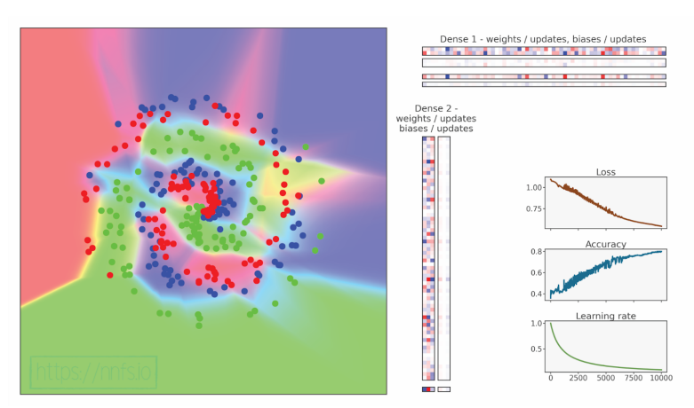
此外，我们准备了动画来帮助可视化训练过程并传达各种优化器及其超参数的影响。动画画布的左侧包含点，其中颜色代表数据的3个类别，坐标是特征，背景颜色显示模型预测区域。理想情况下，点的颜色和背景应该匹配，如果模型分类正确的话。周围区域也应该遵循数据的“趋势”——这就是我们所说的泛化——模型正确预测未见数据的能力。右侧的彩色方块显示权重和偏置——红色代表正值，蓝色代表负值。位于Dense 1条下方和紧邻Dense 2条的相应区域显示优化器对层的更新。更新可能看起来比权重和偏置强得多，但这是因为我们已将它们视觉上标准化为最大值，否则由于更新每次都相当小，它们几乎是看不见的。其他三个图表显示了与训练时间相关的损失、准确率和当前学习率值，在这种情况下是时代。

在这里插入图片描述

我们的神经网络损失值大多停留在1左右，后来是0.85-0.9，准确率大约为0.60。动画还有一种“闪烁摇摆”的效果，这很可能意味着我们选择了过高的学习率。鉴于损失几乎没有减少，我们可以假设这个学习率太高，也导致模型陷入了局部最小值，我们很快将了解更多。在这一点上，迭代更多的时代似乎没有帮助，这告诉我们我们可能被我们的优化卡住了。这是否意味着这是我们能从优化器在这个数据集上得到的最多的东西？

回想一下，我们通过应用某个分数（在这种情况下是1.0）来调整权重和偏差，并从权重和偏差中减去这个分数。这个分数被称为学习率（LR），是优化器减少损失时的主要可调参数。为了获得调整、规划或最初设置学习率的直觉，我们首先应该理解学习率如何影响优化器和损失函数的输出。

代码可视化：https://nnfs.io/pup

2. 学习率（Learning Rate）

到目前为止，我们已经得到了模型及其损失函数对所有参数的梯度，我们希望将这个梯度的一部分应用到参数上以降低损失值。

在大多数情况下，我们不会直接应用负梯度，因为函数最陡下降的方向会持续变化，而且这些值通常对于模型的有效改进来说太大了。相反，我们希望进行小步调整——计算梯度，通过负梯度的一部分更新参数，并在循环中重复这个过程。小步骤确保我们遵循最陡峭的下降方向，但这些步骤也可能太小，导致学习停滞——我们很快会解释这一点。

暂时忘记我们正在执行一个 n 维函数（我们的损失函数）的梯度下降，其中 n 是模型包含的参数（权重和偏置）数量，假设我们的损失函数只有一个维度（单一输入）。我们接下来的图像和动画的目标是可视化一些概念并获得直观理解；因此，我们不会使用或展示某些优化器设置，而是将以更一般的术语考虑问题。也就是说，我们已经使用了一个真实的 SGD 优化器在一个真实的函数上准备了所有以下的示例。这里是我们想要确定输入到它的什么会产生最低可能输出的函数：

在这里插入图片描述

我们可以看到这个函数的全局最小值，即这个函数可能输出的最低 y 值。这是目标——最小化函数的输出以找到全局最小值。在这种情况下，轴的值并不重要。目标仅是展示函数和学习率的概念。同时，请记住，这个一维函数的例子仅用于帮助可视化。使用比解决神经网络的更大的 n 维损失函数所需的数学更简单的方法来解决这个函数将会很容易，其中 n（即权重和偏置的数量）可以达到百万甚至十亿（或更多）。当我们有百万或更多维度时，梯度下降是寻找全局最小值的最著名方法。

我们将从这个图表的左侧开始下降。以一个示例学习率：

在这里插入图片描述

代码可视化：https://nnfs.io/and

学习率太小了。参数的小幅更新导致模型学习停滞——模型卡在了局部最小值。局部最小值是在我们查找附近的最小值，但不一定是全局最小值，全局最小值是函数的绝对最低点。在这里的例子以及优化完整神经网络时，我们不知道全局最小值在哪里。我们如何知道我们是否已经达到全局最小值或至少接近了呢？损失函数衡量模型的预测与真实目标值的接近程度，因此，只要损失值不是0或非常接近0，而且模型停止学习，我们就处于某个局部最小值。实际上，我们几乎从未接近损失值0，这是由于各种原因。其中一个原因可能是神经网络超参数不完善。另一个原因可能是数据不足。如果你的神经网络达到了0的损失值，你应该对此感到怀疑，我们将在本书后面的内容中讨论这些原因。

我们可以尝试修改学习率：

在这里插入图片描述

代码可视化：https://nnfs.io/xor

这一次，模型摆脱了这个局部最小值，但却陷入了另一个局部最小值。让我们再看一个学习率变化后的例子：

在这里插入图片描述

代码可视化：https://nnfs.io/tho

这一次，模型卡在了一个接近全局最小值的局部最小值处。模型能够逃离更“深”的局部最小值，因此它为什么会在这里卡住可能会让人感觉不符合直觉。记住，无论下降有多大或多小，模型都遵循损失函数最陡峭的下降方向。因此，我们将引入动量和其他技术来防止此类情况。

在优化器中，动量增加了梯度，这在物理世界中我们可以称之为惯性（inertia）——例如，我们可以把一个球扔向山坡上，如果山坡足够小或施加的力足够大，球可以滚过山坡的另一边。让我们看看这可能在模型训练中是怎样的：

在这里插入图片描述

代码可视化：https://nnfs.io/pog

在这里，我们使用了非常小的学习率和较大的动量。颜色从绿色、橙色变为红色展示了梯度下降过程的进展，也就是步骤。我们可以看到，模型实现了目标并找到了全局最小值，但这需要许多步骤。这可以做得更好吗？

在这里插入图片描述

代码可视化：https://nnfs.io/jog

甚至更进一步：

在这里插入图片描述

代码可视化：https://nnfs.io/mog

通过调整学习率和动量，我们分别在大约200步、100步和50步内找到了全局最小值。通过调整优化器的参数，可以显著缩短训练时间。然而，我们必须小心这些超参数的调整，因为这并不总是能帮助模型：

在这里插入图片描述

代码可视化：https://nnfs.io/log

当学习率设定过高时，模型可能无法找到全局最小值。甚至在某些时候，如果它确实找到了，进一步的调整可能会导致它跳出这个最小值。我们将在本章稍后看到这种行为——请仔细观察结果，看看你是否能发现我们描述的问题，以及当我们逐一讨论不同的优化器时所遇到的其他问题。

在这种情况下，模型在某个最小值周围“跳动”，这可能意味着我们应该尝试降低学习率、提高动量，或者可能应用学习率衰减（在训练期间降低学习率），我们将在本章中描述这个方法。如果我们将学习率设定得过高：

在这里插入图片描述

代码可视化：https://nnfs.io/sog

在这种情况下，模型开始在周围“跳动”，并以我们可能观察到的随机方向移动。这是一个“超调”的例子，每一步的改变方向是正确的，但应用的梯度量太大了。在极端情况下，我们可能导致梯度爆炸：

在这里插入图片描述

代码可视化：https://nnfs.io/bog

梯度爆炸是一种情况，其中参数更新导致函数的输出上升而不是下降，并且，每一步中，损失值和梯度都会变得更大。在某个点上，由于浮点变量的限制，它无法再容纳这种大小的值，导致溢出，模型将无法继续训练。在训练过程中识别这种情况形成是至关重要的，尤其是对于大型模型，其训练可能需要数天、数周甚至更长时间。及时调整模型的超参数是有可能的，以保存模型并继续训练。

当我们正确选择学习率和其他超参数时，学习过程可以相对较快：

在这里插入图片描述

代码可视化：https://nnfs.io/cog

这一次，模型找到全局最小值所需的时间大大减少，但它总能做得更好：

在这里插入图片描述

代码可视化：https://nnfs.io/rog

这次模型只需要几步就能找到全局最小值。挑战在于正确选择超参数，这并不总是一项容易的任务。通常最好从优化器的默认设置开始，执行几个步骤，调整不同的设置时观察训练过程。在短时间内看到有意义的结果并不总是可能的，在这种情况下，能够在训练期间更新优化器的设置是很好的。如何选择学习率和其他超参数取决于模型、数据，包括数据量、参数初始化方法等。没有单一最佳方式来设置超参数，但经验通常会有所帮助。正如我们提到的，训练神经网络模型的一个挑战是选择正确的设置。不同设置的影响可能从模型根本不学习到学习得非常好都有可能。

关于学习率的总结——如果我们沿着步骤轴绘制损失图：

在这里插入图片描述

我们可以看到各种不同的相对学习率的例子，以及理想情况下，随着训练时间（步数）的增加，损失如何在图表上表现出来。

要知道什么样的学习率能让你的训练过程发挥最大效用是不可能的，但一个好的规则是，你的初期训练将从较大的学习率中受益，以便更快地进行初步步骤。如果你以太小的步骤开始，你可能会陷入局部最小值，并且由于没有对参数进行足够大的更新，你可能无法离开它。

例如，如果我们将SGD优化器的学习率设为0.85而不是1.0会怎样？

# Create dataset
X, y = spiral_data(samples=100, classes=3)

# Create Dense layer with 2 input features and 64 output values
dense1 = Layer_Dense(2, 64)

# Create ReLU activation (to be used with Dense layer):
activation1 = Activation_ReLU()

# Create second Dense layer with 64 input features (as we take output
# of previous layer here) and 3 output values (output values)
dense2 = Layer_Dense(64, 3)

# Create Softmax classifier's combined loss and activation
loss_activation = Activation_Softmax_Loss_CategoricalCrossentropy()

# Create optimizer
learning_rate=.85
optimizer = Optimizer_SGD(learning_rate=learning_rate)

# Train in loop
for epoch in range(10001):
    # Perform a forward pass of our training data through this layer
    dense1.forward(X)
    
    # Perform a forward pass through activation function
    # takes the output of first dense layer here
    activation1.forward(dense1.output)
    
    # Perform a forward pass through second Dense layer
    # takes outputs of activation function of first layer as inputs
    dense2.forward(activation1.output)
    
    # Perform a forward pass through the activation/loss function
    # takes the output of second dense layer here and returns loss
    loss = loss_activation.forward(dense2.output, y)
    
    # Calculate accuracy from output of activation2 and targets
    # calculate values along first axis
    predictions = np.argmax(loss_activation.output, axis=1)
    if len(y.shape) == 2:
    	y = np.argmax(y, axis=1)
    accuracy = np.mean(predictions==y)
    
    if not epoch % 100:
        print(f'epoch: {epoch}, ' +
              f'acc: {accuracy:.3f}, ' +
              f'loss: {loss:.3f}')
    
    # Backward pass
    loss_activation.backward(loss_activation.output, y)
    dense2.backward(loss_activation.dinputs)
    activation1.backward(dense2.dinputs)
    dense1.backward(activation1.dinputs)
    
    # Update weights and biases
    optimizer.update_params(dense1)
    optimizer.update_params(dense2)

>>>
>>>
epoch: 0, acc: 0.360, loss: 1.099
epoch: 100, acc: 0.403, loss: 1.091
...
epoch: 2000, acc: 0.407, loss: 1.037
epoch: 2100, acc: 0.440, loss: 1.027
epoch: 2200, acc: 0.457, loss: 1.038
epoch: 2300, acc: 0.447, loss: 1.042
epoch: 2400, acc: 0.537, loss: 0.986
epoch: 2500, acc: 0.427, loss: 1.009
epoch: 2600, acc: 0.487, loss: 1.029
epoch: 2700, acc: 0.530, loss: 0.986
...
epoch: 7100, acc: 0.567, loss: 0.917
epoch: 7200, acc: 0.587, loss: 0.969
epoch: 7300, acc: 0.553, loss: 0.947
epoch: 7400, acc: 0.610, loss: 0.953
epoch: 7500, acc: 0.573, loss: 0.953
epoch: 7600, acc: 0.537, loss: 0.935
epoch: 7700, acc: 0.547, loss: 0.979
...
epoch: 9100, acc: 0.583, loss: 0.929
epoch: 9200, acc: 0.583, loss: 0.929
...
epoch: 10000, acc: 0.603, loss: 0.942

在这里插入图片描述

代码可视化：https://nnfs.io/cup

正如你所看到的，神经网络在准确性方面并没有提高，而且损失也没有变的更好；但是我们要记住，较低的损失并不总是与更高的准确性相关联。 记住，即使我们希望我们的模型达到最佳的准确性，优化器的任务是减少损失，而不是直接提高准确性。损失是所有样本损失的平均值，其中一些可能会显著下降，而其他一些可能只会略微上升，同时将它们的预测从正确类别改为错误类别。这会导致总体上较低的平均损失，但同时也会导致更多预测不正确的样本，这同时会降低准确性。这种模型准确性较低的可能原因是它偶然找到了另一个局部最小值——由于采取了较小的步骤，下降路径发生了变化。在这两个模型的直接比较训练中，不同的学习率并没有显示出这个学习率值越低越好。在大多数情况下，我们希望从较大的学习率开始，并随着时间/步骤逐渐降低学习率。

一个常用的解决方案是实施学习率衰减，以保持初始更新的大幅度并在训练期间探索各种学习率。

3. 学习率衰减（Learning Rate Decay）

学习率衰减的概念是从较大的学习率开始，例如我们的案例中是1.0，然后在训练过程中逐渐减小它。有几种方法可以做到这一点。其中一种是根据跨越多个训练周期的损失来降低学习率——例如，如果损失开始趋于平稳/达到平台期或开始“跳跃”大幅度变化。你可以逻辑地编程监控这种行为，或者简单地跟踪随时间的损失并在你认为适当时手动降低学习率。另一个选项，我们将要实施的，是编程一个衰减率，它会稳定地按每个批次或周期降低学习率。

我们计划按步骤衰减。这也可以称为1/t衰减或指数衰减。基本上，我们将在每个步骤中按步数的倒数更新学习率。这个倒数是我们将添加到优化器中的一个新的超参数，称为学习率衰减。衰减的工作原理是它取步骤和衰减比例并将它们相乘。训练越深入，步骤就越大，这个乘积的结果也就越大。然后我们取其倒数（训练越深入，该值就越低）并将初始学习率乘以它。添加的1确保最终算法永远不会提高学习率。例如，对于第一步，我们可能会用学习率除以1，例如0.001，这将导致当前学习率为1000。这绝对不是我们想要的。1除以1+比例确保结果，即起始学习率的一部分，始终小于或等于1，随时间减小。这是期望的结果——从当前学习率开始，随时间使其变小。确定当前衰减率的代码如下：

starting_learning_rate = 1.
learning_rate_decay = 0.1
step = 1

learning_rate = starting_learning_rate * (1. / (1 + learning_rate_decay * step))

print(learning_rate)

>>>
0.9090909090909091

在实践中，0.1 会被认为是一个相当激进的衰减率，但这应该能让你对这一概念有所了解。如果我们在第 20 步：

starting_learning_rate = 1.
learning_rate_decay = 0.1
step = 20

learning_rate = starting_learning_rate * (1. / (1 + learning_rate_decay * step))

print(learning_rate)

>>>
0.9090909090909091

我们还可以在一个循环中进行模拟，这与我们应用学习率衰减的方式更为相似：

starting_learning_rate = 1.
learning_rate_decay = 0.1

for step in range(20):
    learning_rate = starting_learning_rate * (1. / (1 + learning_rate_decay * step))
    
    print(learning_rate)

>>>
1.0
0.9090909090909091
0.8333333333333334
0.7692307692307692
0.7142857142857143
0.6666666666666666
0.625
0.588235294117647
0.5555555555555556
0.5263157894736842
0.5
0.47619047619047616
0.45454545454545453
0.4347826086956522
0.41666666666666663
0.4
0.3846153846153846
0.37037037037037035
0.35714285714285715
0.3448275862068965

这种学习率衰减方案通过上述公式在每个步骤中降低学习率。最初，学习率下降很快，但每个步骤中学习率的变化都在减小，让模型尽可能接近最小值。模型在训练结束时需要小的更新，以便尽可能接近这一点。我们现在可以更新我们的SGD优化器类，以允许学习率衰减：

# SGD optimizer        
class Optimizer_SGD:
    # Initialize optimizer - set settings,
    # learning rate of 1. is default for this optimizer
    def __init__(self, learning_rate=1.0, decay=0.):
        self.learning_rate = learning_rate
        self.current_learning_rate = learning_rate
        self.decay = decay
        self.iterations = 0
        
    # Call once before any parameter updates
    def pre_update_params(self):
        if self.decay:
            self.current_learning_rate = self.learning_rate * (1. / (1. + self.decay * self.iterations))
    
    # Update parameters
    def update_params(self, layer):
        layer.weights += -self.learning_rate * layer.dweights
        layer.biases += -self.learning_rate * layer.dbiases
        
    # Call once after any parameter updates
    def post_update_params(self):
        self.iterations += 1

我们在SGD类中更新了一些内容。首先，在__init__方法中，我们添加了对当前学习率的处理，self.learning_rate现在是初始学习率。我们还添加了跟踪衰减率和优化器已经经过的迭代次数的属性。接下来，我们添加了一个名为pre_update_params的新方法。如果我们有一个不为0的衰减率，这个方法将使用前面的公式更新我们的self.current_learning_rate。update_params方法保持不变，但我们有一个新的post_update_params方法，将增加我们的self.iterations跟踪。使用我们更新的SGD优化器类，我们添加了打印当前学习率的功能，并添加了优化器方法的前置和后置调用。让我们使用1e-2（0.01）的衰减率再次训练我们的模型：

# Create dataset
X, y = spiral_data(samples=100, classes=3)

# Create Dense layer with 2 input features and 64 output values
dense1 = Layer_Dense(2, 64)

# Create ReLU activation (to be used with Dense layer):
activation1 = Activation_ReLU()

# Create second Dense layer with 64 input features (as we take output
# of previous layer here) and 3 output values (output values)
dense2 = Layer_Dense(64, 3)

# Create Softmax classifier's combined loss and activation
loss_activation = Activation_Softmax_Loss_CategoricalCrossentropy()

# Create optimizer
# learning_rate=0.85
decay = 1e-2
optimizer = Optimizer_SGD(decay=decay)

# Train in loop
for epoch in range(10001):
    # Perform a forward pass of our training data through this layer
    dense1.forward(X)
    
    # Perform a forward pass through activation function
    # takes the output of first dense layer here
    activation1.forward(dense1.output)
    
    # Perform a forward pass through second Dense layer
    # takes outputs of activation function of first layer as inputs
    dense2.forward(activation1.output)
    
    # Perform a forward pass through the activation/loss function
    # takes the output of second dense layer here and returns loss
    loss = loss_activation.forward(dense2.output, y)
    
    # Calculate accuracy from output of activation2 and targets
    # calculate values along first axis
    predictions = np.argmax(loss_activation.output, axis=1)
    if len(y.shape) == 2:
    	y = np.argmax(y, axis=1)
    accuracy = np.mean(predictions==y)
    
    if not epoch % 100:
        print(f'epoch: {epoch}, ' +
              f'acc: {accuracy:.3f}, ' +
              f'loss: {loss:.3f}, ' +
              f'lr: {optimizer.current_learning_rate}')
    
    # Backward pass
    loss_activation.backward(loss_activation.output, y)
    dense2.backward(loss_activation.dinputs)
    activation1.backward(dense2.dinputs)
    dense1.backward(activation1.dinputs)
    
   # Update weights and biases
    optimizer.pre_update_params()
    optimizer.update_params(dense1)
    optimizer.update_params(dense2)
    optimizer.post_update_params()

>>>
epoch: 0, acc: 0.360, loss: 1.099, lr: 1.0
epoch: 100, acc: 0.400, loss: 1.087, lr: 0.5025125628140703
epoch: 200, acc: 0.417, loss: 1.077, lr: 0.33444816053511706
epoch: 300, acc: 0.420, loss: 1.076, lr: 0.2506265664160401
epoch: 400, acc: 0.400, loss: 1.074, lr: 0.2004008016032064
epoch: 500, acc: 0.400, loss: 1.071, lr: 0.1669449081803005
epoch: 600, acc: 0.417, loss: 1.067, lr: 0.14306151645207438
epoch: 700, acc: 0.437, loss: 1.062, lr: 0.1251564455569462
epoch: 800, acc: 0.430, loss: 1.055, lr: 0.11123470522803114
epoch: 900, acc: 0.390, loss: 1.064, lr: 0.10010010010010009
epoch: 1000, acc: 0.400, loss: 1.062, lr: 0.09099181073703366
...
epoch: 2000, acc: 0.403, loss: 1.037, lr: 0.047641734159123386
...
epoch: 3000, acc: 0.543, loss: 0.985, lr: 0.03226847370119393
...
epoch: 4000, acc: 0.520, loss: 0.971, lr: 0.02439619419370578
...
epoch: 5000, acc: 0.510, loss: 0.973, lr: 0.019611688566385566
...
epoch: 7000, acc: 0.593, loss: 0.905, lr: 0.014086491055078181
...
epoch: 10000, acc: 0.647, loss: 0.874, lr: 0.009901970492127933

在这里插入图片描述

代码可视化：https://nnfs.io/zuk

这个模型肯定卡住了，原因几乎可以肯定是因为学习率衰减得太快，变得太小，使得模型陷入了某个局部最小值。这很可能是为什么我们的准确率和损失不再有任何变化，而不是摆动的原因。

我们可以尝试通过将衰减率设为一个更小的数字来稍微慢一些地进行衰减。例如，我们可以尝试1e-3（0.001）：

# Create dataset
X, y = spiral_data(samples=100, classes=3)

# Create Dense layer with 2 input features and 64 output values
dense1 = Layer_Dense(2, 64)

# Create ReLU activation (to be used with Dense layer):
activation1 = Activation_ReLU()

# Create second Dense layer with 64 input features (as we take output
# of previous layer here) and 3 output values (output values)
dense2 = Layer_Dense(64, 3)

# Create Softmax classifier's combined loss and activation
loss_activation = Activation_Softmax_Loss_CategoricalCrossentropy()

# Create optimizer
# learning_rate=0.85
decay = 1e-3
optimizer = Optimizer_SGD(decay=decay)

# Train in loop
for epoch in range(10001):
    # Perform a forward pass of our training data through this layer
    dense1.forward(X)
    
    # Perform a forward pass through activation function
    # takes the output of first dense layer here
    activation1.forward(dense1.output)
    
    # Perform a forward pass through second Dense layer
    # takes outputs of activation function of first layer as inputs
    dense2.forward(activation1.output)
    
    # Perform a forward pass through the activation/loss function
    # takes the output of second dense layer here and returns loss
    loss = loss_activation.forward(dense2.output, y)
    
    # Calculate accuracy from output of activation2 and targets
    # calculate values along first axis
    predictions = np.argmax(loss_activation.output, axis=1)
    if len(y.shape) == 2:
    	y = np.argmax(y, axis=1)
    accuracy = np.mean(predictions==y)
    
    if not epoch % 100:
        print(f'epoch: {epoch}, ' +
              f'acc: {accuracy:.3f}, ' +
              f'loss: {loss:.3f}, ' +
              f'lr: {optimizer.current_learning_rate}')
    
    # Backward pass
    loss_activation.backward(loss_activation.output, y)
    dense2.backward(loss_activation.dinputs)
    activation1.backward(dense2.dinputs)
    dense1.backward(activation1.dinputs)
    
   # Update weights and biases
    optimizer.pre_update_params()
    optimizer.update_params(dense1)
    optimizer.update_params(dense2)
    optimizer.post_update_params()

>>>
epoch: 0, acc: 0.360, loss: 1.099, lr: 1.0
epoch: 100, acc: 0.400, loss: 1.087, lr: 0.9099181073703367
epoch: 200, acc: 0.417, loss: 1.077, lr: 0.8340283569641367
...
epoch: 1700, acc: 0.397, loss: 1.043, lr: 0.3705075954057058
epoch: 1800, acc: 0.450, loss: 1.038, lr: 0.35727045373347627
epoch: 1900, acc: 0.483, loss: 1.025, lr: 0.3449465332873405
epoch: 2000, acc: 0.403, loss: 1.037, lr: 0.33344448149383127
epoch: 2100, acc: 0.457, loss: 1.022, lr: 0.32268473701193934
...
epoch: 3200, acc: 0.487, loss: 0.976, lr: 0.23815194093831865
...
epoch: 5000, acc: 0.510, loss: 0.973, lr: 0.16669444907484582
...
epoch: 6000, acc: 0.490, loss: 0.940, lr: 0.1428775539362766
...
epoch: 8000, acc: 0.617, loss: 0.874, lr: 0.11112345816201799
...
epoch: 9800, acc: 0.600, loss: 0.926, lr: 0.09260116677470137
epoch: 9900, acc: 0.610, loss: 0.915, lr: 0.09175153683824203
epoch: 10000, acc: 0.647, loss: 0.874, lr: 0.09091735612328393

在这里插入图片描述

代码可视化：https://nnfs.io/muk

我们还应该有可能找到能带来更好结果的参数。例如，你可能会怀疑初始学习率太高。尝试找到更好的设置可以成为一个很好的练习。随意尝试！

带学习率衰减的随机梯度下降可以做得相当好，但仍然是一种基本的优化方法，它只遵循梯度，没有任何可能帮助模型找到损失函数全局最小值的额外逻辑。改善SGD优化器的一个选项是引入动量。

4. 带动量的随机梯度下降法（Stochastic Gradient Descent with Momentum）

动量会创建一个在一定更新次数上的梯度滚动平均值，并在每一步使用这个平均值和独特的梯度。另一种理解这个概念的方式是想象一个球沿着山坡向下滚动——即使它找到了一个小洞或小山丘，动量也会让它直接穿过，向着更低的极小值——这个山丘的底部。这在你被困在某个局部最小值（一个洞）中，并且来回反弹的情况下很有帮助。有了动量，模型更有可能穿过局部最小值，进一步减少损失。简单地说，动量可能仍然指向全局梯度下降的方向。

回想一下本章开头的情形：

在这里插入图片描述

在常规更新中，SGD优化器可能会认为下一个最佳步骤是让模型保持在局部最小值中。请记住，梯度指向该步骤当前最陡的损失上升方向——取梯度向量的负值会将其翻转向当前最陡的下降方向，这并不一定意味着朝向全局最小值下降——当前最陡的下降可能指向一个局部最小值。因此，这一步可能会降低该更新的损失，但可能无法让我们摆脱局部最小值。我们可能会遇到一个指向一个方向的梯度，然后在下一个更新中指向相反方向；梯度可能继续在局部最小值周围来回反弹，使损失优化停滞不前。相反，动量使用前一次更新的方向来影响下一次更新的方向，最小化反复回弹和陷入困境的机会。

回顾本章中的另一个例子：

在这里插入图片描述

我们通过设置一个介于0到1之间的参数来利用动量，该参数表示保留前一次参数更新的一部分的比例，并从中减去（添加负值）实际梯度与学习率的乘积（与之前一样）。更新中包含了前几步梯度的一部分作为动量（前几次变化的方向）以及当前梯度的一部分；这两部分共同构成了对参数的实际更新。如果动量在更新中占据的比例较大，更新方向的变化速度会变得更慢。当我们将动量比例设置得过高时，模型可能完全停止学习，因为更新的方向将无法跟随全局梯度下降。其代码如下：

weight_updates = self.momentum * layer.weight_momentums - self.current_learning_rate * layer.dweights

超参数 self.momentum 在开始时被选择，且 layer.weight_momentums 初始值全为零，但在训练过程中会发生变化。

layer.weight_momentums = weight_updates

这意味着动量始终是对参数的上一次更新。我们将对偏置执行与上述相同的操作。然后，我们可以在 SGD 优化器类的 update_params 方法中加入动量计算，将其应用于参数，并将其保留用于下一步，作为当前代码的一种替代操作链。不同之处在于，我们仅计算更新，并将这些更新添加到通用代码中：

# Update parameters
def update_params(self, layer):
    # If we use momentum
    if self.momentum:
        # If layer does not contain momentum arrays, create them
        # filled with zeros
        if not hasattr(layer, 'weight_momentums'):
            layer.weight_momentums = np.zeros_like(layer.weights)
            # If there is no momentum array for weights
            # The array doesn't exist for biases yet either.
            layer.bias_momentums = np.zeros_like(layer.biases)
        # Build weight updates with momentum - take previous
        # updates multiplied by retain factor and update with
        # current gradients
        weight_updates = self.momentum * layer.weight_momentums - self.current_learning_rate * layer.dweights
        layer.weight_momentums = weight_updates
        # Build bias updates
        bias_updates = self.momentum * layer.bias_momentums - self.current_learning_rate * layer.dbiases
        layer.bias_momentums = bias_updates
    # Vanilla SGD updates (as before momentum update)
    else:
        weight_updates = -self.current_learning_rate * layer.dweights
        bias_updates = -self.current_learning_rate * layer.dbiases
    # Update weights and biases using either
    # vanilla or momentum updates
    layer.weights += weight_updates
    layer.biases += bias_updates

制作我们完整的 SGD 优化类：

# SGD optimizer        
class Optimizer_SGD:
    # Initialize optimizer - set settings,
    # learning rate of 1. is default for this optimizer
    def __init__(self, learning_rate=1.0, decay=0., momentum=0.):
        self.learning_rate = learning_rate
        self.current_learning_rate = learning_rate
        self.decay = decay
        self.iterations = 0
        self.momentum = momentum
        
    # Call once before any parameter updates
    def pre_update_params(self):
        if self.decay:
            self.current_learning_rate = self.learning_rate * (1. / (1. + self.decay * self.iterations))
    
    # Update parameters
    def update_params(self, layer):
        # If we use momentum
        if self.momentum:
            # If layer does not contain momentum arrays, create them
            # filled with zeros
            if not hasattr(layer, 'weight_momentums'):
                layer.weight_momentums = np.zeros_like(layer.weights)
                # If there is no momentum array for weights
                # The array doesn't exist for biases yet either.
                layer.bias_momentums = np.zeros_like(layer.biases)
            # Build weight updates with momentum - take previous
            # updates multiplied by retain factor and update with
            # current gradients
            weight_updates = self.momentum * layer.weight_momentums - self.current_learning_rate * layer.dweights
            layer.weight_momentums = weight_updates
            # Build bias updates
            bias_updates = self.momentum * layer.bias_momentums - self.current_learning_rate * layer.dbiases
            layer.bias_momentums = bias_updates
        # Vanilla SGD updates (as before momentum update)
        else:
            weight_updates = -self.current_learning_rate * layer.dweights
            bias_updates = -self.current_learning_rate * layer.dbiases
        # Update weights and biases using either
        # vanilla or momentum updates
        layer.weights += weight_updates
        layer.biases += bias_updates
        
    # Call once after any parameter updates
    def post_update_params(self):
        self.iterations += 1

让我们通过一个例子来展示添加动量如何改变学习过程。保持与之前训练尝试相同的初始学习率（1）和衰减率（1e-3），并使用动量为0.5：

# Create dataset
X, y = spiral_data(samples=100, classes=3)

# Create Dense layer with 2 input features and 64 output values
dense1 = Layer_Dense(2, 64)

# Create ReLU activation (to be used with Dense layer):
activation1 = Activation_ReLU()

# Create second Dense layer with 64 input features (as we take output
# of previous layer here) and 3 output values (output values)
dense2 = Layer_Dense(64, 3)

# Create Softmax classifier's combined loss and activation
loss_activation = Activation_Softmax_Loss_CategoricalCrossentropy()

# Create optimizer
optimizer = Optimizer_SGD(decay=1e-3, momentum=0.5)

# Train in loop
for epoch in range(10001):
    # Perform a forward pass of our training data through this layer
    dense1.forward(X)
    
    # Perform a forward pass through activation function
    # takes the output of first dense layer here
    activation1.forward(dense1.output)
    
    # Perform a forward pass through second Dense layer
    # takes outputs of activation function of first layer as inputs
    dense2.forward(activation1.output)
    
    # Perform a forward pass through the activation/loss function
    # takes the output of second dense layer here and returns loss
    loss = loss_activation.forward(dense2.output, y)
    
    # Calculate accuracy from output of activation2 and targets
    # calculate values along first axis
    predictions = np.argmax(loss_activation.output, axis=1)
    if len(y.shape) == 2:
    	y = np.argmax(y, axis=1)
    accuracy = np.mean(predictions==y)
    
    if not epoch % 100:
        print(f'epoch: {epoch}, ' +
              f'acc: {accuracy:.3f}, ' +
              f'loss: {loss:.3f}, ' +
              f'lr: {optimizer.current_learning_rate}')
    
    # Backward pass
    loss_activation.backward(loss_activation.output, y)
    dense2.backward(loss_activation.dinputs)
    activation1.backward(dense2.dinputs)
    dense1.backward(activation1.dinputs)
    
    # Update weights and biases
    optimizer.pre_update_params()
    optimizer.update_params(dense1)
    optimizer.update_params(dense2)
    optimizer.post_update_params()

>>>
epoch: 0, acc: 0.360, loss: 1.099, lr: 1.0
epoch: 100, acc: 0.427, loss: 1.078, lr: 0.9099181073703367
epoch: 200, acc: 0.420, loss: 1.075, lr: 0.8340283569641367
epoch: 300, acc: 0.407, loss: 1.071, lr: 0.7698229407236336
...
epoch: 1800, acc: 0.547, loss: 0.972, lr: 0.35727045373347627
epoch: 1900, acc: 0.543, loss: 0.964, lr: 0.3449465332873405
...
epoch: 3100, acc: 0.583, loss: 0.885, lr: 0.2439619419370578
epoch: 3200, acc: 0.620, loss: 0.857, lr: 0.23815194093831865
epoch: 3300, acc: 0.603, loss: 0.868, lr: 0.23261223540358225
epoch: 3400, acc: 0.583, loss: 0.881, lr: 0.22732439190725165
...
epoch: 4600, acc: 0.653, loss: 0.766, lr: 0.1786033220217896
epoch: 4700, acc: 0.663, loss: 0.751, lr: 0.1754693805930865
...
epoch: 6000, acc: 0.703, loss: 0.678, lr: 0.1428775539362766
...
epoch: 8000, acc: 0.743, loss: 0.603, lr: 0.11112345816201799
...
epoch: 10000, acc: 0.780, loss: 0.553, lr: 0.09091735612328393

在这里插入图片描述

代码可视化：https://nnfs.io/ram

该模型实现了迄今为止我们所看到的最低损耗和最高精确度，但我们还能做得更好吗？当然可以！让我们试着将动量设置为 0.9：

# Create dataset
X, y = spiral_data(samples=100, classes=3)

# Create Dense layer with 2 input features and 64 output values
dense1 = Layer_Dense(2, 64)

# Create ReLU activation (to be used with Dense layer):
activation1 = Activation_ReLU()

# Create second Dense layer with 64 input features (as we take output
# of previous layer here) and 3 output values (output values)
dense2 = Layer_Dense(64, 3)

# Create Softmax classifier's combined loss and activation
loss_activation = Activation_Softmax_Loss_CategoricalCrossentropy()

# Create optimizer
optimizer = Optimizer_SGD(decay=1e-3, momentum=0.9)

# Train in loop
for epoch in range(10001):
    # Perform a forward pass of our training data through this layer
    dense1.forward(X)
    
    # Perform a forward pass through activation function
    # takes the output of first dense layer here
    activation1.forward(dense1.output)
    
    # Perform a forward pass through second Dense layer
    # takes outputs of activation function of first layer as inputs
    dense2.forward(activation1.output)
    
    # Perform a forward pass through the activation/loss function
    # takes the output of second dense layer here and returns loss
    loss = loss_activation.forward(dense2.output, y)
    
    # Calculate accuracy from output of activation2 and targets
    # calculate values along first axis
    predictions = np.argmax(loss_activation.output, axis=1)
    if len(y.shape) == 2:
    	y = np.argmax(y, axis=1)
    accuracy = np.mean(predictions==y)
    
    if not epoch % 100:
        print(f'epoch: {epoch}, ' +
              f'acc: {accuracy:.3f}, ' +
              f'loss: {loss:.3f}, ' +
              f'lr: {optimizer.current_learning_rate}')
    
    # Backward pass
    loss_activation.backward(loss_activation.output, y)
    dense2.backward(loss_activation.dinputs)
    activation1.backward(dense2.dinputs)
    dense1.backward(activation1.dinputs)
    
    # Update weights and biases
    optimizer.pre_update_params()
    optimizer.update_params(dense1)
    optimizer.update_params(dense2)
    optimizer.post_update_params()

>>>
epoch: 0, acc: 0.360, loss: 1.099, lr: 1.0
epoch: 100, acc: 0.443, loss: 1.053, lr: 0.9099181073703367
epoch: 200, acc: 0.550, loss: 0.955, lr: 0.8340283569641367
epoch: 300, acc: 0.640, loss: 0.763, lr: 0.7698229407236336
epoch: 400, acc: 0.647, loss: 0.732, lr: 0.7147962830593281
epoch: 500, acc: 0.687, loss: 0.666, lr: 0.66711140760507
epoch: 600, acc: 0.757, loss: 0.564, lr: 0.6253908692933083
epoch: 700, acc: 0.787, loss: 0.513, lr: 0.5885815185403178
epoch: 800, acc: 0.730, loss: 0.604, lr: 0.5558643690939411
epoch: 900, acc: 0.833, loss: 0.442, lr: 0.526592943654555
epoch: 1000, acc: 0.837, loss: 0.447, lr: 0.5002501250625312
...
epoch: 2200, acc: 0.913, loss: 0.249, lr: 0.31259768677711786
...
epoch: 2900, acc: 0.920, loss: 0.196, lr: 0.25647601949217746
...
epoch: 3800, acc: 0.940, loss: 0.162, lr: 0.20837674515524068
...
epoch: 7100, acc: 0.947, loss: 0.132, lr: 0.12347203358439313
...
epoch: 10000, acc: 0.957, loss: 0.121, lr: 0.09091735612328393

在这里插入图片描述

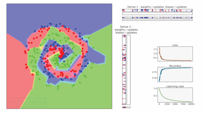
代码可视化：https://nnfs.io/map

这是一个足够好的例子，说明动量如何能够发挥作用。模型在前1000个周期中达到了接近84%的准确率，并进一步提升，最终以95.7%的准确率和0.121的损失结束。这些结果是一个很大的改进。带有动量的 SGD 优化器在实际应用中通常是两种主要优化器选择之一，另一种是我们稍后会讨论的 Adam 优化器。在此之前，我们还有另外两种优化器需要讨论。接下来对随机梯度下降的修改是 AdaGrad。

5. 自适应梯度（adaptive gradient：AdaGrad）

AdaGrad（全称为自适应梯度）为每个参数引入了独立的学习率，而不是全局共享的学习率。其核心思想是对特征的更新进行归一化。在训练过程中，某些权重可能会显著上升，而其他权重变化较小。通常，最好是权重之间的差异不要过大，这一点我们将在正则化技术中进一步讨论。AdaGrad 通过保留先前更新的历史记录来实现参数更新的归一化——如果更新的总和（无论是正还是负）越大，那么在后续训练中进行的更新就越小。这使得更新频率较低的参数能够跟上变化，从而更有效地利用更多的神经元进行训练。AdaGrad 的概念可以用以下两行代码来概括：

cache += parm_gradient ** 2
parm_updates = learning_rate * parm_gradient / (sqrt(cache) + eps)

缓存保存了梯度平方的历史，而参数更新 parm_updates 是学习率乘以梯度（到目前为止是基本的 SGD）然后除以缓存的平方根加上一个 $\epsilon$ 值的函数。由于缓存值的不断增加，这种除法操作可能会导致学习停滞，因为随着时间推移，更新变得越来越小，这是因为更新的单调性质。这也是为什么该优化器并不广泛使用，除非在某些特定的应用中。 $\epsilon$ 是一个超参数（预训练时的控制参数设置），用于防止分母为0的情况。 $\epsilon$ 的值通常是一个很小的数，例如 1e-7，这是我们将默认采用的值。你可能还会注意到，我们在累加平方值后又计算了平方根，这看起来可能有些违背直觉，不理解为什么要这么做。我们累加的是平方值并取平方根，而这与直接累加值并不相同，例如：

在这里插入图片描述

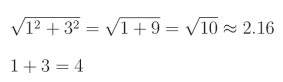
最终的缓存值增长得更慢，并且以不同的方式增长，同时处理了负数的情况（我们不希望用负数来除以更新值并反转其符号）。总体而言，对于梯度较小的参数，其学习率会缓慢下降，而对于梯度较大的参数，其学习率下降得更快。为了实现 AdaGrad，我们首先复制粘贴 SGD 优化器类，更改类名，在 init 方法中添加一个 $\epsilon$ 属性，默认值为 1e-7，并移除动量相关的代码。接下来，在 update_params 方法中，我们将替换动量代码为：

# Update parameters
def update_params(self, layer): 
    # If layer does not contain cache arrays,
    # create them filled with zeros
    if not hasattr(layer, 'weight_cache'):
        layer.weight_cache = np.zeros_like(layer.weights)
        layer.bias_cache = np.zeros_like(layer.biases)
    # Update cache with squared current gradients
    layer.weight_cache += layer.dweights**2
    layer.bias_cache += layer.dbiases**2
    # Vanilla SGD parameter update + normalization
    # with square rooted cache
    layer.weights += -self.current_learning_rate * layer.dweights / (np.sqrt(layer.weight_cache) + self.epsilon)
    layer.biases += -self.current_learning_rate * layer.dbiases / (np.sqrt(layer.bias_cache) + self.epsilon)

我们添加了缓存及其更新逻辑，然后将更新值除以缓存的平方根。以下是完整的 AdaGrad 优化器代码：

# Adagrad optimizer
class Optimizer_Adagrad:
    # Initialize optimizer - set settings
    def __init__(self, learning_rate=1., decay=0., epsilon=1e-7):
        self.learning_rate = learning_rate
        self.current_learning_rate = learning_rate
        self.decay = decay
        self.iterations = 0
        self.epsilon = epsilon
        
    # Call once before any parameter updates
    def pre_update_params(self):
        if self.decay:
            self.current_learning_rate = self.learning_rate * (1. / (1. + self.decay * self.iterations))
    
    # Update parameters
    def update_params(self, layer):
        # If layer does not contain cache arrays,
        # create them filled with zeros
        if not hasattr(layer, 'weight_cache'):
            layer.weight_cache = np.zeros_like(layer.weights)
            layer.bias_cache = np.zeros_like(layer.biases)
        # Update cache with squared current gradients
        layer.weight_cache += layer.dweights**2
        layer.bias_cache += layer.dbiases**2
        # Vanilla SGD parameter update + normalization
        # with square rooted cache
        layer.weights += -self.current_learning_rate * layer.dweights / (np.sqrt(layer.weight_cache) + self.epsilon)
        layer.biases += -self.current_learning_rate * layer.dbiases / (np.sqrt(layer.bias_cache) + self.epsilon)
        
    # Call once after any parameter updates
    def post_update_params(self):
        self.iterations += 1

现在使用衰减设置为 1e-4 和 1e-5 的优化器进行测试，比我们之前使用的 1e-3 效果更好。使用我们的数据集时，该优化器在衰减较小的情况下效果更好：

# Create dataset
X, y = spiral_data(samples=100, classes=3)

# Create Dense layer with 2 input features and 64 output values
dense1 = Layer_Dense(2, 64)

# Create ReLU activation (to be used with Dense layer):
activation1 = Activation_ReLU()

# Create second Dense layer with 64 input features (as we take output
# of previous layer here) and 3 output values (output values)
dense2 = Layer_Dense(64, 3)

# Create Softmax classifier's combined loss and activation
loss_activation = Activation_Softmax_Loss_CategoricalCrossentropy()

# Create optimizer
# optimizer = Optimizer_SGD(decay=8e-8, momentum=0.9)
optimizer = Optimizer_Adagrad(decay=1e-4)

# Train in loop
for epoch in range(10001):
    # Perform a forward pass of our training data through this layer
    dense1.forward(X)
    
    # Perform a forward pass through activation function
    # takes the output of first dense layer here
    activation1.forward(dense1.output)
    
    # Perform a forward pass through second Dense layer
    # takes outputs of activation function of first layer as inputs
    dense2.forward(activation1.output)
    
    # Perform a forward pass through the activation/loss function
    # takes the output of second dense layer here and returns loss
    loss = loss_activation.forward(dense2.output, y)
    
    # Calculate accuracy from output of activation2 and targets
    # calculate values along first axis
    predictions = np.argmax(loss_activation.output, axis=1)
    if len(y.shape) == 2:
    	y = np.argmax(y, axis=1)
    accuracy = np.mean(predictions==y)
    
    if not epoch % 100:
        print(f'epoch: {epoch}, ' +
              f'acc: {accuracy:.3f}, ' +
              f'loss: {loss:.3f}, ' +
              f'lr: {optimizer.current_learning_rate}')
    
    # Backward pass
    loss_activation.backward(loss_activation.output, y)
    dense2.backward(loss_activation.dinputs)
    activation1.backward(dense2.dinputs)
    dense1.backward(activation1.dinputs)
    
    # Update weights and biases
    optimizer.pre_update_params()
    optimizer.update_params(dense1)
    optimizer.update_params(dense2)
    optimizer.post_update_params()

>>>
epoch: 0, acc: 0.360, loss: 1.099, lr: 1.0
epoch: 100, acc: 0.453, loss: 1.011, lr: 0.9901970492127933
epoch: 200, acc: 0.530, loss: 0.935, lr: 0.9804882831650161
epoch: 300, acc: 0.613, loss: 0.868, lr: 0.9709680551509855
epoch: 400, acc: 0.623, loss: 0.830, lr: 0.9616309260505818
epoch: 500, acc: 0.617, loss: 0.793, lr: 0.9524716639679969
...
epoch: 1200, acc: 0.703, loss: 0.638, lr: 0.892936869363336
...
epoch: 1700, acc: 0.777, loss: 0.578, lr: 0.8547739123001966
...
epoch: 4700, acc: 0.813, loss: 0.463, lr: 0.6803183890060548
...
epoch: 5100, acc: 0.813, loss: 0.455, lr: 0.6622955162593549
...
epoch: 6700, acc: 0.833, loss: 0.422, lr: 0.5988382537876519
...
epoch: 7500, acc: 0.840, loss: 0.410, lr: 0.5714612263557918
...
epoch: 9900, acc: 0.837, loss: 0.385, lr: 0.5025378159706518
epoch: 10000, acc: 0.840, loss: 0.385, lr: 0.5000250012500626

在这里插入图片描述

代码可视化：https://nnfs.io/bop

AdaGrad 在这里表现得相当不错，但不如带动量的 SGD 效果好。从整个训练过程中可以看到，损失值一直在持续下降。有趣的是，AdaGrad 最初需要多花费几个周期才能达到与带动量的随机梯度下降（Stochastic Gradient Descent with momentum）相似的结果。

6. 均方根传播（Root Mean Square Propagation：RMSProp）

继续探讨随机梯度下降（Stochastic Gradient Descent）的改进方法，我们来到了 RMSProp，全称为均方根传播（Root Mean Square Propagation）。与 AdaGrad 类似，RMSProp 为每个参数计算自适应学习率，只是其计算方式与 AdaGrad 不同。

AdaGrad 的缓存计算公式为：

cache += gradient ** 2

RMSProp 计算高速缓存的方式为：

cache = rho * cache + (1 - rho) * gradient **  2

请注意，这种方法类似于带动量的 SGD 优化器和 AdaGrad 的缓存机制。RMSProp 添加了一种类似于动量的机制，同时还引入了每个参数的自适应学习率，使学习率的变化更加平滑。这有助于保持变化的全局方向，同时减缓方向的改变。与 AdaGrad 持续将梯度平方累加到缓存不同，RMSProp 使用缓存的移动平均值。每次更新缓存时，保留一部分旧缓存，并用新梯度平方的一部分进行更新。通过这种方式，缓存内容随时间和数据变化移动，避免学习过程停滞。在这种优化器中，每个参数的学习率可以根据最近的更新和当前的梯度而上升或下降。RMSProp 以与 AdaGrad 相同的方式应用缓存。

# RMSprop optimizer
class Optimizer_RMSprop:
    # Initialize optimizer - set settings
    def __init__(self, learning_rate=0.001, decay=0., epsilon=1e-7, rho=0.9):
        self.learning_rate = learning_rate
        self.current_learning_rate = learning_rate
        self.decay = decay
        self.iterations = 0
        self.epsilon = epsilon
        self.rho = rho

    # Call once before any parameter updates
    def pre_update_params(self):
        if self.decay:
            self.current_learning_rate = self.learning_rate * (1. / (1. + self.decay * self.iterations))
            
    # Update parameters
    def update_params(self, layer):
        # If layer does not contain cache arrays,
        # create them filled with zeros
        if not hasattr(layer, 'weight_cache'):
            layer.weight_cache = np.zeros_like(layer.weights)
            layer.bias_cache = np.zeros_like(layer.biases)
        # Update cache with squared current gradients
        layer.weight_cache = self.rho * layer.weight_cache + (1 - self.rho) * layer.dweights**2
        layer.bias_cache = self.rho * layer.bias_cache + (1 - self.rho) * layer.dbiases**2
        # Vanilla SGD parameter update + normalization
        # with square rooted cache
        layer.weights += -self.current_learning_rate * layer.dweights / (np.sqrt(layer.weight_cache) + self.epsilon)
        layer.biases += -self.current_learning_rate * layer.dbiases / (np.sqrt(layer.bias_cache) + self.epsilon)

    # Call once after any parameter updates
    def post_update_params(self):
        self.iterations += 1

更改主要神经网络测试代码中使用的优化器：

optimizer = Optimizer_RMSprop(decay=1e-4)

运行这段代码后，我们可以：

>>>
epoch: 0, acc: 0.360, loss: 1.099, lr: 0.001
epoch: 100, acc: 0.437, loss: 1.077, lr: 0.0009901970492127933
epoch: 200, acc: 0.457, loss: 1.072, lr: 0.0009804882831650162
epoch: 300, acc: 0.473, loss: 1.062, lr: 0.0009709680551509856
...
epoch: 1000, acc: 0.600, loss: 0.961, lr: 0.0009091735612328393
...
epoch: 4800, acc: 0.693, loss: 0.766, lr: 0.0006757213325224677
...
epoch: 5800, acc: 0.697, loss: 0.742, lr: 0.0006329514526235838
...
epoch: 7100, acc: 0.717, loss: 0.716, lr: 0.0005848295221942804
...
epoch: 10000, acc: 0.730, loss: 0.666, lr: 0.0005000250012500625

在这里插入图片描述

代码可视化：https://nnfs.io/pun

结果并不理想，但我们可以稍微调整一下超参数：

optimizer = Optimizer_RMSprop(learning_rate=0.02, decay=1e-5, rho=0.999)

>>>
epoch: 0, acc: 0.360, loss: 1.099, lr: 0.02
epoch: 100, acc: 0.467, loss: 1.013, lr: 0.01998021958261321
epoch: 200, acc: 0.533, loss: 0.960, lr: 0.019960279044701046
...
epoch: 600, acc: 0.657, loss: 0.764, lr: 0.019880913329158343
...
epoch: 1000, acc: 0.730, loss: 0.637, lr: 0.019802176259170884
...
epoch: 1800, acc: 0.813, loss: 0.480, lr: 0.01964655841412981
...
epoch: 3800, acc: 0.830, loss: 0.359, lr: 0.01926800836231563
...
epoch: 6200, acc: 0.867, loss: 0.281, lr: 0.018832569044906263
...
epoch: 6600, acc: 0.893, loss: 0.255, lr: 0.018761902081633034
...
epoch: 7100, acc: 0.893, loss: 0.265, lr: 0.018674310684506857
...
epoch: 9500, acc: 0.900, loss: 0.239, lr: 0.018265006986365174
epoch: 9600, acc: 0.897, loss: 0.241, lr: 0.018248341681949654
epoch: 9700, acc: 0.900, loss: 0.240, lr: 0.018231706761228456
epoch: 9800, acc: 0.907, loss: 0.221, lr: 0.018215102141185255
epoch: 9900, acc: 0.900, loss: 0.238, lr: 0.018198527739105907
epoch: 10000, acc: 0.900, loss: 0.238, lr: 0.018181983472577025

在这里插入图片描述

代码可视化：https://nnfs.io/not

结果相当不错，接近带动量的 SGD，但没有那么好。我们还需要对随机梯度下降进行最后一次调整。

7. 自适应动量优化器（Adaptive Momentum：Adam）

Adam（全称为自适应动量优化器，Adaptive Momentum）是当前最广泛使用的优化器，它建立在 RMSProp 的基础之上，并重新引入了 SGD 的动量概念。这意味着我们不会直接应用当前的梯度，而是像带动量的 SGD 优化器一样应用动量，然后结合 RMSProp 的缓存机制，为每个权重应用自适应学习率。

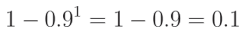
Adam 优化器额外添加了一个偏差校正机制。请不要将此与层的偏置混淆。偏差校正机制应用于缓存和动量，用于补偿初始零值在训练的最初阶段尚未“热启动”的情况。为了实现这一校正，动量和缓存都需要除以 $1-\beta^{step}$ 。随着步数（ $s t e p$ ）的增加， $\beta^{step}$ 趋近于0（一个分数的指数随着值增加而减少），从而使整个表达式在初期阶段为一个分数，并随着训练的进行逐渐接近1。

例如， $\beta 1$ （用于应用动量的分数）的默认值为 $0.9$ 。这意味着在第一步时，校正值等于：

在这里插入图片描述

随着训练的进展，步数也会增加：

在这里插入图片描述

同样的机制也适用于缓存（ $c a c h e$ ）和 $\beta 2$ 。在这种情况下， $\beta 2$ 的初始值为 $0.001$ ，并且随着训练的进行逐渐接近1。这些值分别用于除以动量（ $m o m e n t u m s$ ）和缓存。用一个小于1的分数除法会使它们的值增加数倍，从而显著加速训练的初始阶段，直到经过多次初始步骤后动量和缓存逐渐“热启动”。我们之前还提到，这两个偏差校正系数（bias-correcting coefficients）在训练过程中会趋向于1，使参数更新在后期训练阶段恢复到通常的值。为了获得参数更新，我们将缩放后的动量除以缩放后的平方根缓存。

Adam 优化器的代码基于 RMSProp 优化器。它添加了从 SGD 优化器引入的缓存机制以及超参数 $\beta 1$ ，并引入了动量和缓存的偏差校正机制。此外，我们还修改了参数更新的计算方式——使用校正后的动量和缓存，而不是梯度和缓存。以下是从 RMSProp 优化器改动的完整清单，列于下面的代码之后：

# Adam optimizer
class Optimizer_Adam:
    # Initialize optimizer - set settings
    def __init__(self, learning_rate=0.001, decay=0., epsilon=1e-7, beta_1=0.9, beta_2=0.999):
        self.learning_rate = learning_rate
        self.current_learning_rate = learning_rate
        self.decay = decay
        self.iterations = 0
        self.epsilon = epsilon
        self.beta_1 = beta_1
        self.beta_2 = beta_2

    # Call once before any parameter updates
    def pre_update_params(self):
        if self.decay:
            self.current_learning_rate = self.learning_rate * (1. / (1. + self.decay * self.iterations))

    # Update parameters
    def update_params(self, layer):
        # If layer does not contain cache arrays,
        # create them filled with zeros
        if not hasattr(layer, 'weight_cache'):
            layer.weight_momentums = np.zeros_like(layer.weights)
            layer.weight_cache = np.zeros_like(layer.weights)
            layer.bias_momentums = np.zeros_like(layer.biases)
            layer.bias_cache = np.zeros_like(layer.biases)
        # Update momentum with current gradients
        layer.weight_momentums = self.beta_1 * layer.weight_momentums + (1 - self.beta_1) * layer.dweights
        layer.bias_momentums = self.beta_1 * layer.bias_momentums + (1 - self.beta_1) * layer.dbiases
        # Get corrected momentum
        # self.iteration is 0 at first pass
        # and we need to start with 1 here
        weight_momentums_corrected = layer.weight_momentums / (1 - self.beta_1 ** (self.iterations + 1))
        bias_momentums_corrected = layer.bias_momentums / (1 - self.beta_1 ** (self.iterations + 1))
        # Update cache with squared current gradients
        layer.weight_cache = self.beta_2 * layer.weight_cache + (1 - self.beta_2) * layer.dweights**2
        layer.bias_cache = self.beta_2 * layer.bias_cache + (1 - self.beta_2) * layer.dbiases**2
        # Get corrected cache
        weight_cache_corrected = layer.weight_cache / (1 - self.beta_2 ** (self.iterations + 1))
        bias_cache_corrected = layer.bias_cache / (1 - self.beta_2 ** (self.iterations + 1))
        # Vanilla SGD parameter update + normalization
        # with square rooted cache
        layer.weights += -self.current_learning_rate * weight_momentums_corrected / (np.sqrt(weight_cache_corrected) + self.epsilon)
        layer.biases += -self.current_learning_rate * bias_momentums_corrected / (np.sqrt(bias_cache_corrected) + self.epsilon)

    # Call once after any parameter updates
    def post_update_params(self):
        self.iterations += 1

从 RMSProp 类代码复制后，我们进行了以下改动：

将类名从 Optimizer_RMSprop 重命名为 Optimizer_Adam。
在 __init__ 中将超参数和属性名称从 rho 重命名为 beta_2。
在 __init__ 中新增超参数 beta_1 和对应的属性。
在 update_params() 方法中添加 $m o m e n t u m$ 数组的创建。
添加 $m o m e n t u m$ 的计算逻辑。
在 update_params 方法中的缓存计算代码中，将 self.rho 重命名为 self.beta_2。
添加了 *_corrected 变量，用于表示校正后的动量和权重。
在参数更新中，用包含动量数组的校正值替换了 layer.dweights、layer.dbiases、layer.weight_cache 和 layer.bias_cache。

回到我们的主神经网络代码，现在我们可以将优化器设置为 Adam，运行代码，并观察这些改动带来了怎样的影响：

optimizer = Optimizer_Adam(learning_rate=0.02, decay=1e-5)

按照默认设置，我们的结果是：

>>>
epoch: 0, acc: 0.360, loss: 1.099, lr: 0.02
epoch: 100, acc: 0.673, loss: 0.769, lr: 0.01998021958261321
epoch: 200, acc: 0.813, loss: 0.552, lr: 0.019960279044701046
epoch: 300, acc: 0.840, loss: 0.445, lr: 0.019940378268975763
epoch: 400, acc: 0.863, loss: 0.380, lr: 0.01992051713662487
epoch: 500, acc: 0.873, loss: 0.336, lr: 0.01990069552930875
epoch: 600, acc: 0.890, loss: 0.308, lr: 0.019880913329158343
epoch: 700, acc: 0.890, loss: 0.287, lr: 0.019861170418772778
...
epoch: 1700, acc: 0.937, loss: 0.184, lr: 0.019665876753950384
...
epoch: 2600, acc: 0.947, loss: 0.142, lr: 0.019493367381748363
...
epoch: 9900, acc: 0.967, loss: 0.082, lr: 0.018198527739105907
epoch: 10000, acc: 0.963, loss: 0.081, lr: 0.018181983472577025

在这里插入图片描述

代码可视化：https://nnfs.io/you

这是目前最好的结果，但我们还是把学习率调高一点，调到 0.05，并把衰减改为 5e-7：

optimizer = Optimizer_Adam(learning_rate=0.05, decay=5e-7)

在这种情况下，损耗和精确度略有提高，最终结束：

>>>
epoch: 0, acc: 0.360, loss: 1.099, lr: 0.05
epoch: 100, acc: 0.670, loss: 0.705, lr: 0.04999752512250644
epoch: 200, acc: 0.797, loss: 0.522, lr: 0.04999502549496326
...
epoch: 700, acc: 0.917, loss: 0.252, lr: 0.049982531105378675
epoch: 800, acc: 0.920, loss: 0.245, lr: 0.04998003297682575
epoch: 900, acc: 0.930, loss: 0.228, lr: 0.049977535097973466
...
epoch: 2000, acc: 0.947, loss: 0.151, lr: 0.04995007490013731
...
epoch: 3300, acc: 0.960, loss: 0.117, lr: 0.04991766081847992
...
epoch: 7800, acc: 0.960, loss: 0.082, lr: 0.04980578235171948
epoch: 7900, acc: 0.963, loss: 0.081, lr: 0.04980330185930667
epoch: 8000, acc: 0.963, loss: 0.081, lr: 0.04980082161395499
...
epoch: 9900, acc: 0.963, loss: 0.074, lr: 0.049753743844839965
epoch: 10000, acc: 0.967, loss: 0.074, lr: 0.04975126853296942

在这里插入图片描述

代码可视化：https://nnfs.io/car

在准确率和损失方面，Adam 的表现并没有显著提高。虽然 Adam 在这里表现最佳，且通常是这些优化器中效果最好的，但这并不总是如此。通常建议先尝试 Adam 优化器，但如果结果不如预期，也应该尝试其他优化器，特别是简单的 SGD 或 SGD + 动量，有时它们的表现会优于 Adam。原因可能各不相同，但需要牢记这一点。

我们稍后会讨论训练时如何选择各种超参数（例如学习率）。对于 SGD，一个通用的初始学习率是 $1.0$ ，衰减至 $0.1$ 。对于 Adam，一个好的初始学习率是 $0.001$ （1e-3），衰减至 $0.0001$ （1e-4）。不同的问题可能需要不同的数值，但这些是不错的起始值。

在本节中，我们在生成的数据集上达到了 $98.3\%$ 的准确率，并且损失值接近完美（ $0$ ）。然而，与其兴奋，不如谨慎对待这样的结果。你将很快学会对如此优秀的结果保持警惕，或者至少以谨慎的态度接近它们。有些情况下，确实可以获得如此优异的有效结果，但在本例中，我们忽略了机器学习中的一个重要概念：样本外测试数据（out-of-sample testing data），它可以揭示过拟合的问题。这将是下一节的主题。

到此为止的全部代码：

import numpy as np
from timeit import timeit
import nnfs
from nnfs.datasets import spiral_data

nnfs.init()

# Dense layer
class Layer_Dense:
    # Layer initialization
    def __init__(self, inputs, neurons):
        # Initialize weights and biases
        self.weights = 0.01 * np.random.randn(inputs, neurons)
        self.biases = np.zeros((1, neurons))
        
    # Forward pass
    def forward(self, inputs):
        # Remember input values
        self.inputs = inputs
        # Calculate output values from inputs, weights and biases
        self.output = np.dot(inputs, self.weights) + self.biases

    # Backward pass
    def backward(self, dvalues):
        # Gradients on parameters
        self.dweights = np.dot(self.inputs.T, dvalues)
        self.dbiases = np.sum(dvalues, axis=0, keepdims=True)
        # Gradient on values
        self.dinputs = np.dot(dvalues, self.weights.T)
        
        
# ReLU activation
class Activation_ReLU:
    # Forward pass
    def forward(self, inputs):
        # Remember input values
        self.inputs = inputs
        # Calculate output values from inputs
        self.output = np.maximum(0, inputs)
        
    # Backward pass
    def backward(self, dvalues):
        # Since we need to modify the original variable,
        # let's make a copy of the values first
        self.dinputs = dvalues.copy()
        # Zero gradient where input values were negative
        self.dinputs[self.inputs <= 0] = 0
        
        
# Softmax activation
class Activation_Softmax:
    # Forward pass
    def forward(self, inputs):
        # Remember input values
        self.inputs = inputs
        # Get unnormalized probabilities
        exp_values = np.exp(inputs - np.max(inputs, axis=1, 
                                            keepdims=True))
        # Normalize them for each sample
        probabilities = exp_values / np.sum(exp_values, axis=1, 
                                            keepdims=True)
        self.output = probabilities
        
    # Backward pass
    def backward(self, dvalues):
        # Create uninitialized array
        self.dinputs = np.empty_like(dvalues)
        # Enumerate outputs and gradients
        for index, (single_output, single_dvalues) in enumerate(zip(self.output, dvalues)):
            # Flatten output array
            single_output = single_output.reshape(-1, 1)
            # Calculate Jacobian matrix of the output and
            jacobian_matrix = np.diagflat(single_output) - np.dot(single_output, single_output.T)
            # Calculate sample-wise gradient
            # and add it to the array of sample gradients
            self.dinputs[index] = np.dot(jacobian_matrix, single_dvalues)
            

# Common loss class
class Loss:
    # Calculates the data and regularization losses
    # given model output and ground truth values
    def calculate(self, output, y):
        # Calculate sample losses
        sample_losses = self.forward(output, y)
        # Calculate mean loss
        data_loss = np.mean(sample_losses)
        # Return loss
        return data_loss
    
    
# Cross-entropy loss
class Loss_CategoricalCrossentropy(Loss):
    # Forward pass
    def forward(self, y_pred, y_true):
        # Number of samples in a batch
        samples = len(y_pred)
        # Clip data to prevent division by 0
        # Clip both sides to not drag mean towards any value
        y_pred_clipped = np.clip(y_pred, 1e-7, 1 - 1e-7)
        # Probabilities for target values -
        # only if categorical labels
        if len(y_true.shape) == 1:
            correct_confidences = y_pred_clipped[range(samples), y_true]
        # Mask values - only for one-hot encoded labels
        elif len(y_true.shape) == 2:
            correct_confidences = np.sum(y_pred_clipped * y_true, axis=1)
        # Losses
        negative_log_likelihoods = -np.log(correct_confidences)
        return negative_log_likelihoods
    
    # Backward pass
    def backward(self, dvalues, y_true):
        # Number of samples
        samples = len(dvalues)
        # Number of labels in every sample
        # We'll use the first sample to count them
        labels = len(dvalues[0])
        # If labels are sparse, turn them into one-hot vector
        if len(y_true.shape) == 1: # check whether they are one-dimensional
            y_true = np.eye(labels)[y_true]
        # Calculate gradient
        self.dinputs = -y_true / dvalues
        # Normalize gradient
        self.dinputs = self.dinputs / samples
        
        
# Softmax classifier - combined Softmax activation
# and cross-entropy loss for faster backward step
class Activation_Softmax_Loss_CategoricalCrossentropy():
    # Creates activation and loss function objects
    def __init__(self):
        self.activation = Activation_Softmax()
        self.loss = Loss_CategoricalCrossentropy()
        
    # Forward pass
    def forward(self, inputs, y_true):
        # Output layer's activation function
        self.activation.forward(inputs)
        # Set the output
        self.output = self.activation.output
        # Calculate and return loss value
        return self.loss.calculate(self.output, y_true)
    
    # Backward pass
    def backward(self, dvalues, y_true):
        # Number of samples
        samples = len(dvalues)
        # If labels are one-hot encoded,
        # turn them into discrete values
        if len(y_true.shape) == 2:
            y_true = np.argmax(y_true, axis=1)
        # Copy so we can safely modify
        self.dinputs = dvalues.copy()
        # Calculate gradient
        self.dinputs[range(samples), y_true] -= 1
        # Normalize gradient
        self.dinputs = self.dinputs / samples
        
        
# SGD optimizer        
class Optimizer_SGD:
    # Initialize optimizer - set settings,
    # learning rate of 1. is default for this optimizer
    def __init__(self, learning_rate=1.0, decay=0., momentum=0.):
        self.learning_rate = learning_rate
        self.current_learning_rate = learning_rate
        self.decay = decay
        self.iterations = 0
        self.momentum = momentum
        
    # Call once before any parameter updates
    def pre_update_params(self):
        if self.decay:
            self.current_learning_rate = self.learning_rate * (1. / (1. + self.decay * self.iterations))
    
    # Update parameters
    def update_params(self, layer):
        # If we use momentum
        if self.momentum:
            # If layer does not contain momentum arrays, create them
            # filled with zeros
            if not hasattr(layer, 'weight_momentums'):
                layer.weight_momentums = np.zeros_like(layer.weights)
                # If there is no momentum array for weights
                # The array doesn't exist for biases yet either.
                layer.bias_momentums = np.zeros_like(layer.biases)
            # Build weight updates with momentum - take previous
            # updates multiplied by retain factor and update with
            # current gradients
            weight_updates = self.momentum * layer.weight_momentums - self.current_learning_rate * layer.dweights
            layer.weight_momentums = weight_updates
            # Build bias updates
            bias_updates = self.momentum * layer.bias_momentums - self.current_learning_rate * layer.dbiases
            layer.bias_momentums = bias_updates
        # Vanilla SGD updates (as before momentum update)
        else:
            weight_updates = -self.current_learning_rate * layer.dweights
            bias_updates = -self.current_learning_rate * layer.dbiases
        # Update weights and biases using either
        # vanilla or momentum updates
        layer.weights += weight_updates
        layer.biases += bias_updates
        
    # Call once after any parameter updates
    def post_update_params(self):
        self.iterations += 1
        
        
# Adagrad optimizer
class Optimizer_Adagrad:
    # Initialize optimizer - set settings
    def __init__(self, learning_rate=1., decay=0., epsilon=1e-7):
        self.learning_rate = learning_rate
        self.current_learning_rate = learning_rate
        self.decay = decay
        self.iterations = 0
        self.epsilon = epsilon
        
    # Call once before any parameter updates
    def pre_update_params(self):
        if self.decay:
            self.current_learning_rate = self.learning_rate * (1. / (1. + self.decay * self.iterations))
    
    # Update parameters
    def update_params(self, layer):
        # If layer does not contain cache arrays,
        # create them filled with zeros
        if not hasattr(layer, 'weight_cache'):
            layer.weight_cache = np.zeros_like(layer.weights)
            layer.bias_cache = np.zeros_like(layer.biases)
        # Update cache with squared current gradients
        layer.weight_cache += layer.dweights**2
        layer.bias_cache += layer.dbiases**2
        # Vanilla SGD parameter update + normalization
        # with square rooted cache
        layer.weights += -self.current_learning_rate * layer.dweights / (np.sqrt(layer.weight_cache) + self.epsilon)
        layer.biases += -self.current_learning_rate * layer.dbiases / (np.sqrt(layer.bias_cache) + self.epsilon)
        
    # Call once after any parameter updates
    def post_update_params(self):
        self.iterations += 1


# RMSprop optimizer
class Optimizer_RMSprop:
    # Initialize optimizer - set settings
    def __init__(self, learning_rate=0.001, decay=0., epsilon=1e-7, rho=0.9):
        self.learning_rate = learning_rate
        self.current_learning_rate = learning_rate
        self.decay = decay
        self.iterations = 0
        self.epsilon = epsilon
        self.rho = rho

    # Call once before any parameter updates
    def pre_update_params(self):
        if self.decay:
            self.current_learning_rate = self.learning_rate * (1. / (1. + self.decay * self.iterations))
            
    # Update parameters
    def update_params(self, layer):
        # If layer does not contain cache arrays,
        # create them filled with zeros
        if not hasattr(layer, 'weight_cache'):
            layer.weight_cache = np.zeros_like(layer.weights)
            layer.bias_cache = np.zeros_like(layer.biases)
        # Update cache with squared current gradients
        layer.weight_cache = self.rho * layer.weight_cache + (1 - self.rho) * layer.dweights**2
        layer.bias_cache = self.rho * layer.bias_cache + (1 - self.rho) * layer.dbiases**2
        # Vanilla SGD parameter update + normalization
        # with square rooted cache
        layer.weights += -self.current_learning_rate * layer.dweights / (np.sqrt(layer.weight_cache) + self.epsilon)
        layer.biases += -self.current_learning_rate * layer.dbiases / (np.sqrt(layer.bias_cache) + self.epsilon)

    # Call once after any parameter updates
    def post_update_params(self):
        self.iterations += 1


# Adam optimizer
class Optimizer_Adam:
    # Initialize optimizer - set settings
    def __init__(self, learning_rate=0.001, decay=0., epsilon=1e-7, beta_1=0.9, beta_2=0.999):
        self.learning_rate = learning_rate
        self.current_learning_rate = learning_rate
        self.decay = decay
        self.iterations = 0
        self.epsilon = epsilon
        self.beta_1 = beta_1
        self.beta_2 = beta_2

    # Call once before any parameter updates
    def pre_update_params(self):
        if self.decay:
            self.current_learning_rate = self.learning_rate * (1. / (1. + self.decay * self.iterations))

    # Update parameters
    def update_params(self, layer):
        # If layer does not contain cache arrays,
        # create them filled with zeros
        if not hasattr(layer, 'weight_cache'):
            layer.weight_momentums = np.zeros_like(layer.weights)
            layer.weight_cache = np.zeros_like(layer.weights)
            layer.bias_momentums = np.zeros_like(layer.biases)
            layer.bias_cache = np.zeros_like(layer.biases)
        # Update momentum with current gradients
        layer.weight_momentums = self.beta_1 * layer.weight_momentums + (1 - self.beta_1) * layer.dweights
        layer.bias_momentums = self.beta_1 * layer.bias_momentums + (1 - self.beta_1) * layer.dbiases
        # Get corrected momentum
        # self.iteration is 0 at first pass
        # and we need to start with 1 here
        weight_momentums_corrected = layer.weight_momentums / (1 - self.beta_1 ** (self.iterations + 1))
        bias_momentums_corrected = layer.bias_momentums / (1 - self.beta_1 ** (self.iterations + 1))
        # Update cache with squared current gradients
        layer.weight_cache = self.beta_2 * layer.weight_cache + (1 - self.beta_2) * layer.dweights**2
        layer.bias_cache = self.beta_2 * layer.bias_cache + (1 - self.beta_2) * layer.dbiases**2
        # Get corrected cache
        weight_cache_corrected = layer.weight_cache / (1 - self.beta_2 ** (self.iterations + 1))
        bias_cache_corrected = layer.bias_cache / (1 - self.beta_2 ** (self.iterations + 1))
        # Vanilla SGD parameter update + normalization
        # with square rooted cache
        layer.weights += -self.current_learning_rate * weight_momentums_corrected / (np.sqrt(weight_cache_corrected) + self.epsilon)
        layer.biases += -self.current_learning_rate * bias_momentums_corrected / (np.sqrt(bias_cache_corrected) + self.epsilon)

    # Call once after any parameter updates
    def post_update_params(self):
        self.iterations += 1


# Create dataset
X, y = spiral_data(samples=100, classes=3)

# Create Dense layer with 2 input features and 64 output values
dense1 = Layer_Dense(2, 64)

# Create ReLU activation (to be used with Dense layer):
activation1 = Activation_ReLU()

# Create second Dense layer with 64 input features (as we take output
# of previous layer here) and 3 output values (output values)
dense2 = Layer_Dense(64, 3)

# Create Softmax classifier's combined loss and activation
loss_activation = Activation_Softmax_Loss_CategoricalCrossentropy()

# Create optimizer
# optimizer = Optimizer_SGD(decay=8e-8, momentum=0.9)
# optimizer = Optimizer_RMSprop(decay=1e-4)
# optimizer = Optimizer_RMSprop(learning_rate=0.02, decay=1e-5, rho=0.999)
# optimizer = Optimizer_Adam(learning_rate=0.02, decay=1e-5)
optimizer = Optimizer_Adam(learning_rate=0.05, decay=5e-7)

# Train in loop
for epoch in range(10001):
    # Perform a forward pass of our training data through this layer
    dense1.forward(X)
    
    # Perform a forward pass through activation function
    # takes the output of first dense layer here
    activation1.forward(dense1.output)
    
    # Perform a forward pass through second Dense layer
    # takes outputs of activation function of first layer as inputs
    dense2.forward(activation1.output)
    
    # Perform a forward pass through the activation/loss function
    # takes the output of second dense layer here and returns loss
    loss = loss_activation.forward(dense2.output, y)
    
    # Calculate accuracy from output of activation2 and targets
    # calculate values along first axis
    predictions = np.argmax(loss_activation.output, axis=1)
    if len(y.shape) == 2:
    	y = np.argmax(y, axis=1)
    accuracy = np.mean(predictions==y)
    
    if not epoch % 100:
        print(f'epoch: {epoch}, ' +
              f'acc: {accuracy:.3f}, ' +
              f'loss: {loss:.3f}, ' +
              f'lr: {optimizer.current_learning_rate}')
    
    # Backward pass
    loss_activation.backward(loss_activation.output, y)
    dense2.backward(loss_activation.dinputs)
    activation1.backward(dense2.dinputs)
    dense1.backward(activation1.dinputs)
    
    # Update weights and biases
    optimizer.pre_update_params()
    optimizer.update_params(dense1)
    optimizer.update_params(dense2)
    optimizer.post_update_params()