图示几种基本排序的平均时间效率

本文承接上一篇博客《基本排序算法的C语言实现》而写，主要使用图示分析验证排序算法的时间效率。
首先是排序算法运行20次所需的平均时间与排序元素个数的关系图。

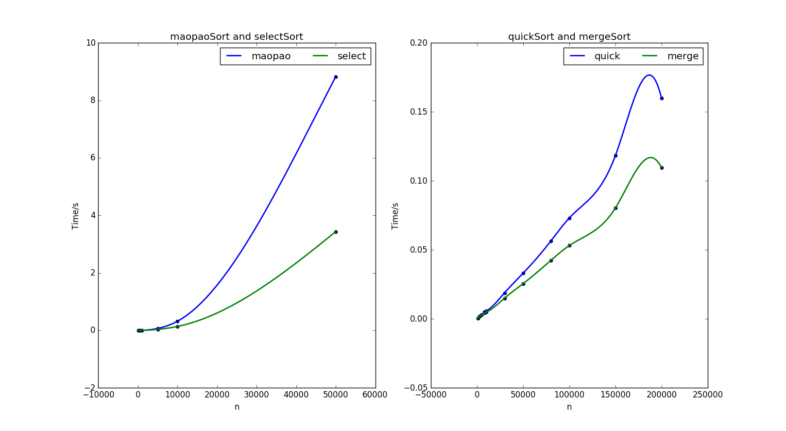
如同事前分析的，冒泡排序与选择排序的运行时间几乎是以n^2增长的，并且选择排序比冒泡排序的系数要小一些。而快排与归并排序的运行时间是以近乎常数级增长的，而图片右端的非正常突起段是由于插值算法引起的。直观的可以感受到，快速排序，归并排序在10^5数量级上仍然可以在10^（-1）秒内得到结果，而冒泡与选择在10^5时，已经让我等的不耐烦了，好像电脑跑了几光年一样。

原始测试数据如下，依次是冒泡，选择，快排，归并。冒泡与选择选用的元素个数集为[100,500,1000,5000,10000,50000],快排与归并选用的元素个数集为[1000,3000,5000,8000,10000,30000,50000,80000,100000,150000,200000]，所用时间如下：

0.000050,0.000650,0.002550,0.067400,0.318050,8.825100
0.000000,0.000350,0.001500,0.034600,0.136350,3.435700
0.000550,0.001800,0.002850,0.004900,0.005700,0.018900,0.033050,0.056350,0.073050,0.118300,0.159900
0.000450,0.001700,0.002750,0.004250,0.004850,0.015050,0.025450,0.042300,0.053100,0.080350,0.109500

绘制图像的Python源码为：

#-*-coding:utf-8-*-
#平均排序时间的图示

import matplotlib.pyplot as plt
import csv
from scipy.interpolate import interp1d
import numpy as np
def load_data(file_path):
    data=[]
    with open(file_path,'r') as ti:
        reader=csv.reader(ti)
        data=[row for row in reader]
    data1=[]
    for item in data:
        dataa=[float(itemm) for itemm in item]
        data1.append(dataa)
    return data1
#数据准备
data= load_data('testReTime.csv')
count1=[100,500,1000,5000,10000,50000]
count2=[1000,3000,5000,8000,10000,30000,50000,80000,100000,150000,200000]
#print data
#数据准备
def picture():
    cubic0_inter=interp1d(count1,data[0],kind='cubic') #创建插值函数
    cubic1_inter=interp1d(count1,data[1],kind='cubic')
    xIndex=np.arange(100,50000,1)
    mY=cubic0_inter(xIndex)
    sY=cubic1_inter(xIndex)
    ax=plt.subplot(121)
    ax.scatter(count1,data[0])
    ax.scatter(count1,data[1])
    ax.plot(xIndex,mY,linewidth=2,label='maopao')
    ax.plot(xIndex,sY,linewidth=2,label='select')
    ax.legend(loc=1,ncol=2)
    ax.set_xlabel('n')
    ax.set_ylabel('Time/s')
    ax.set_title('maopaoSort and selectSort')

    cubic2_inter=interp1d(count2,data[2],kind='cubic') #创建插值函数
    cubic3_inter=interp1d(count2,data[3],kind='cubic')
    xIndex=np.arange(1000,200000,1)
    qY=cubic2_inter(xIndex)
    mmY=cubic3_inter(xIndex)
    ax1=plt.subplot(122)
    ax1.scatter(count2,data[2])
    ax1.scatter(count2,data[3])
    ax1.plot(xIndex,qY,linewidth=2,label='quick')
    ax1.plot(xIndex,mmY,linewidth=2,label='merge')
    ax1.legend(loc=1,ncol=2)
    ax1.set_xlabel('n')
    ax1.set_ylabel('Time/s')
    ax1.set_title('quickSort and mergeSort')

    plt.show()
picture()

欧克，希望这篇博文可以帮助筒子们直观的理解到算法的时间效率是多么重要，算法效率高才是硬道理，欢迎大家转载。