


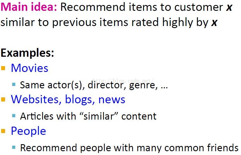
(个性化)推荐系统构建三大方法:基于内容的推荐content-based,协同过滤collaborative filtering,隐语义模型(LFM, latent factor model)推荐。这篇博客主要讲基于内容的推荐content-based。
基于内容的推荐1 Content-based System
{MMDs中基于user-item profile空间的cosin相似度的思路}
主要思想

上图同时使用了explict和impliict信息建立Item profiles,推荐时很可能是推荐红色的六边形。
Item模型 Item Profile
将item表示成一个features向量,如电影的features向量可以是<author, title, actor, director, ...>对应的boolean或者real-valued的数值向量。
这里不同的features数值一般需要scale一下,不然数值偏大的features会dominate整个item模型的表示。其中一个比较公平的选择缩放因子的方法是:使其每个缩放因子与其对应分量的平均值成反比。另一种对向量分量进行放缩变换的方式是首先对向量进行归一化,也就是说计算每个分量的平均值然后对向量中的每一个分量减去对应的平均值。

文章推荐中的item描述示例:Text Features
Profile = set of “important” words in item (document)
使用TF-IDF进行文本特征抽取,所以文本的profile是一个real vector,并且要设置一个threshold来过滤。[Scikit-learn:Feature extraction文本特征提取:TF-IDF(Term frequency * Inverse Doc Frequency)词权重]
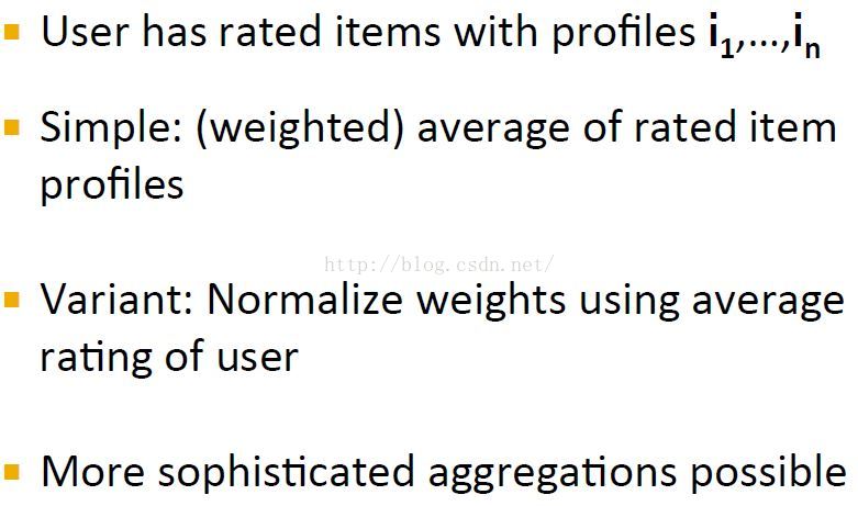
User模型 User Profile
通过用户评分过(或者有过互动如观看)的item的profiles构建用户的profiles。构建用户模型的几种方式:
simple方式建立一个用户profile的一个图示(不过这里还没加上weight):其中每个向量是一个item(如电影)的向量表示(向量分量可以是actor,这样的话分类属性就要用独热编码表示,或者直接每个actor都表示成一个feature)

用户profile建立示例
注意用户的profile向量和item向量是同样的表示,就是说item vec中的元素是profile(e.g actor),user vec中的元素也是profile(e.g actor)。用户的profile是基于评分过的item profile建立的(没有评分的就不用)。效用矩阵(utility matrix)就是user-item矩阵,如评分或者是否观看的boolean矩阵[多个用户是矩阵,一个用户的时候当然就是向量了,下面的例子都是以一个用户来说明的],用户和item之间通过效用矩阵连接:(当然为了方便也可以不显示使用效用矩阵,直接计算用户评分过的电影数据)

示例1:Boolen Utility Matrix(simple方式,无评分,但有观看)


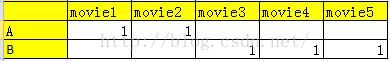
这个实际就是上面的simple方式,所有看过的电影item向量加起来/N。电影的profile就是[(1,0), (1, 0), ....],这样用户的profile就是(0.4, 0.6)。
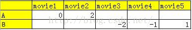
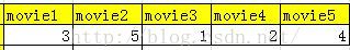
示例2:Star Ratings(variant方式,有评分)


If the utility matrix is not boolean, e.g., ratings 1–5, then we can weight the vectors representing the profiles of items by the utility value.

原始

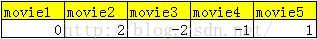
user rating normalized
实际上是分两步的:
先将效用矩阵效用值归一化,作为项表示向量的权重
 =》
=》
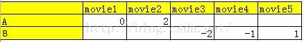
再将项表示向量加权平均:
 =》
=》
 =》
=》
由于每个user的慷慨程度不同,打分的出手值不同,需要规格化。通过规格化发现评分1 和2实际上是negative ratings。
规格化就相当于将item vec的每个属性进行了一个规格化,这种规格化是通过这个属性的所有item进行的。
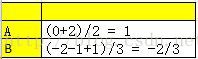
注意profile的均值计算是用户对所有电影评分总分的均值,而profile A的计算是(0+2)/profile A在电影中出现的次数,而不是用户评分的所有电影总数。
这种方式有效的一个直觉知识是:每个Item中的profile评分都减去了总体均值,去除了不同用户的慷慨程度影响,而除以profile在电影中出现的次数相当于再计算一次个体均值,更好拟合对某个profile的偏好程序。
推荐Making Predictions
使用余弦相似度来度量user profile和item profile的相似度,因为它适合高维度向量的相似度计算,且cosin值越大越相似(此时角度就越小)。[ 距离和相似性度量方法]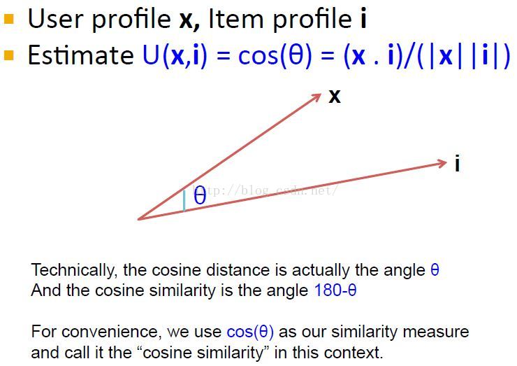
这样,我们就计算用户x的catlog中所有item i进行相似度计算,推荐给用户相似度高的items。
皮皮blog
评价:基于内容推荐的优缺点pros and cons
优点

1 新来item一来就可以作推荐,它的推荐是基于其本身特征,而不是其它用户对其的评分。没有协同过滤的first-rater问题。
2 意味着you can start working making content-based recommendations from day one for your very first user.
3 协同过滤对于口味独特的用户可能找不到相似用户,而基于内容的推荐仍然可以推荐。when we get to collaborative filtering,We need to find similar users.But if the user were very unique or idiosyncratic taste there may not be any other similar users.But the content-based approach, user can very unique tastes as long as we can build item profiles for the items that the user likes.
缺点

如果用户从未评分过某种类型的item,那么那种item也永远不会被推荐给用户,即使那个item在当前是相当受欢迎的。
冷启动问题:新用户没有profile。
[海量数据挖掘Mining Massive Datasets(MMDs) week4-Jure Leskovec courses 推荐系统Recommendation System]
皮皮blog
基于内容的推荐2 Content Based Recommendations
{Andrew NG机器学习course中基于user-item profile线性规划的思路}
基于线性规划的主要思想
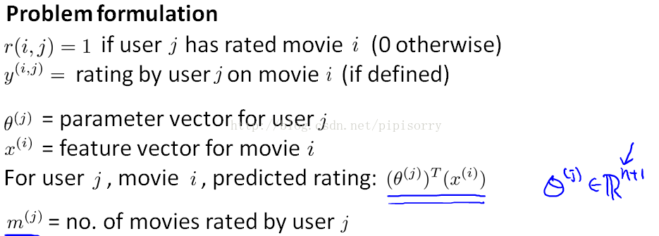
我们将每个用户的评分预测看成一个分开独立的线性回归问题 separate linear regression problem,也就是说对每个用户j我们都要去学习它的参数向量θ^j(维度R=n+1,其中n为features的数目),这样我们就通过内积θj'Xi来预测user j对item i的评分。
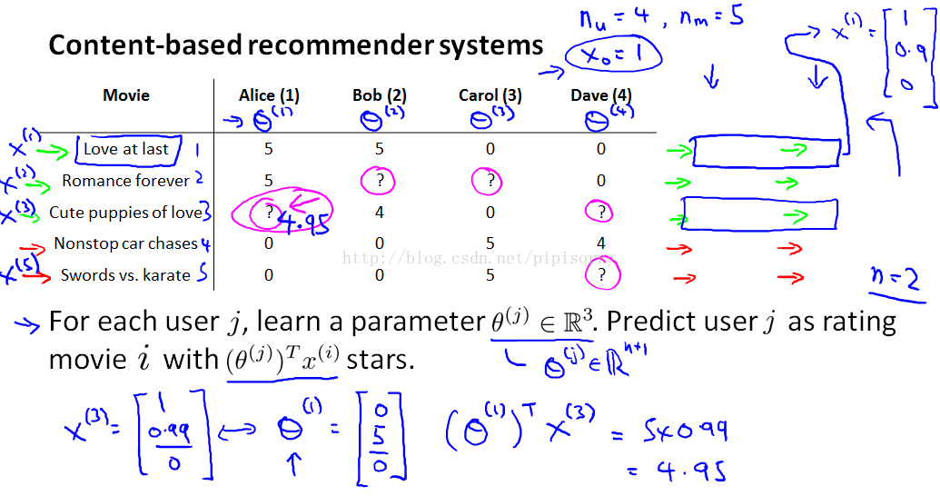
content based recommendations:我们假设我们已经有不同items的features了,that capture what is the content of these movies, how romantic/action is this movie?这样的话我们就是在用items的内容features来作预测。
我们对每个item的feature向量都添加一个额外的截断interceptor feature x0=1,n=2为feature的数目(不包括x0)。
假设我们通过线性规划求出了Alice的参数θ(对于Alice评过的每部电影就是一个example,其中example0中x = [0.9 0], y = 5,用梯度下降求出theta),这样预测Alice对第3部电影的评分为4.95(如图)。
最优化算法:参数向量θj的估计
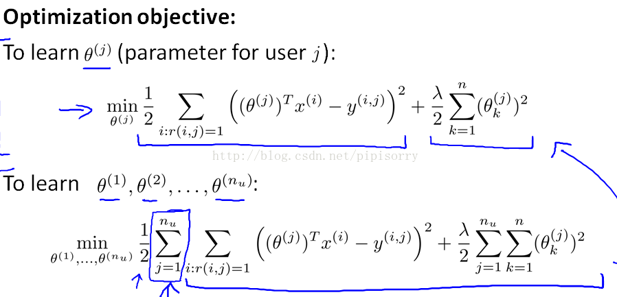

Note: 常数项1/mj删除了;且同线性规划一样不regularize θ0。
Suppose there is only one user and he has rated every movie in the training set. This implies that nu=1 and r(i,j)=1 for every i,j. In this case, the cost function J(θ) is equivalent to the one used for regularized linear regression.
[机器学习Machine Learning - Andrew NG courses]
Reviews复习
规格化问题

计算出规格化后的矩阵为:
[[-1.333 -1. 0. 0.333 2. ]
[-0.333 0. -1. 1.333 0. ]
[ 1.667 1. 1. -1.667 -2. ]]
Content-based的cosin距离计算问题
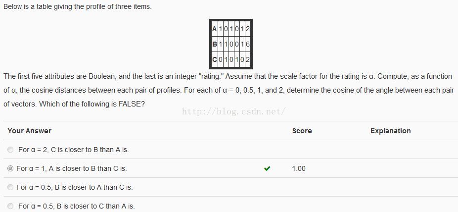
Note: 距离越小越相似。
计算得到的距离矩阵分别为:
scale_alpha = 0 scale_alpha = 0.5 scale_alpha = 1 scale_alpha = 2
A B C A B C A B C A B C
[[ 0. 0.333 1. ] [[ 0. 0.278 0.711] [[ 0. 0.153 0.383] [[ 0. 0.054 0.135]
[ 0.333 0. 0.592] [ 0.278 0. 0.333] [ 0.153 0. 0.15 ] [ 0.054 0. 0.047]
[ 1. 0.592 0. ]] [ 0.711 0.333 0. ]] [ 0.383 0.15 0. ]] [ 0.135 0.047 0. ]]
代码:
import numpy as np
from scipy import spatial

from Utility.PrintOptions import printoptions


def Nomalize(A):
    '''
    user-item规格化:对每个元素先减行和,再减列和
    '''
    row_mean = np.mean(A, 1).reshape([len(A), 1])  # 进行广播运算
    A -= row_mean

    col_mean = np.mean(A, 0)
    A -= col_mean
    with printoptions(precision=3):
        print(A)
    return A


def CosineDist(A, scale_alpha):
    '''
    计算行向量间的cosin相似度
    '''
    A[:, -1] *= scale_alpha
    cos_dist = spatial.distance.squareform(spatial.distance.pdist(A, metric='cosine'))
    with printoptions(precision=3):
        print('scale_alpha = %s' % scale_alpha)
        print('\tA\t\tB\t\tC')
        print(cos_dist)
        print()


if __name__ == '__main__':
    task = 2
    if task == 1:
        A = np.array([[1, 2, 3, 4, 5], [2, 3, 2, 5, 3], [5, 5, 5, 3, 2]], dtype=float)
        Nomalize(A)
    else:
        for scale_alpha in [0, 0.5, 1, 2]:
            A = np.array([[1, 0, 1, 0, 1, 2], [1, 1, 0, 0, 1, 6], [0, 1, 0, 1, 0, 2]], dtype=float)
            CosineDist(A, scale_alpha=scale_alpha)


 1863
1863

 被折叠的 条评论
为什么被折叠?
被折叠的 条评论
为什么被折叠?
 到【灌水乐园】发言


