【图像分类】【深度学习】【轻量级网络】【Pytorch版本】MobileNets_V1模型算法详解

牙牙要健康

已于 2023-12-15 13:42:42 修改

阅读量1.2k

点赞数 2

分类专栏：深度学习图像分类轻量级网络文章标签：深度学习 pytorch

于 2023-04-07 10:50:43 首次发布

本文链接：https://blog.csdn.net/yangyu0515/article/details/129994083

版权

深度学习同时被 3 个专栏收录

69 篇文章 22 订阅

订阅专栏

图像分类

17 篇文章 0 订阅

订阅专栏

轻量级网络

6 篇文章 0 订阅

订阅专栏

【图像分类】【深度学习】【轻量级网络】【Pytorch版本】MobileNets_V1模型算法详解

文章目录

【图像分类】【深度学习】【轻量级网络】【Pytorch版本】MobileNets_V1模型算法详解
前言
MobleNet_V1讲解
MobleNet_V1 Pytorch代码
完整代码
总结

前言

MobileNets_V1是由谷歌公司的Howard, Andrew G等人在《MobileNets: Efficient Convolutional Neural Networks for Mobile Vision Applications【CVPR-2017】》【论文地址】一文中提出的模型，是一种采用了深度可分离卷积的轻量级CNN网络，它将标准卷积分为深度卷积和逐点卷积，更加适用于移动端和边缘计算设备。

MobleNet_V1讲解

Depthwise Separable Convolution(深度可分离卷积)

标准卷积一次性完成滤波和合并过程，产生新的输出。
MobileNet模型是基于深度可分离卷积的，深度可分离卷积则拆解了标准卷积的形式，它将标准卷积拆解为深度卷积和点卷积这俩层，大大减少了计算量和模型大小：

1.深度卷积用于滤波，深度卷积对每个输入通道应用一个单独的滤波器；
2.点卷积用于合并，应用1×1的卷积来合并深度卷积的输出。

下图是根据MobileNets_V1论文绘制的普通卷积的卷积核和深度可分离卷积的卷积核之间的详细示意图：

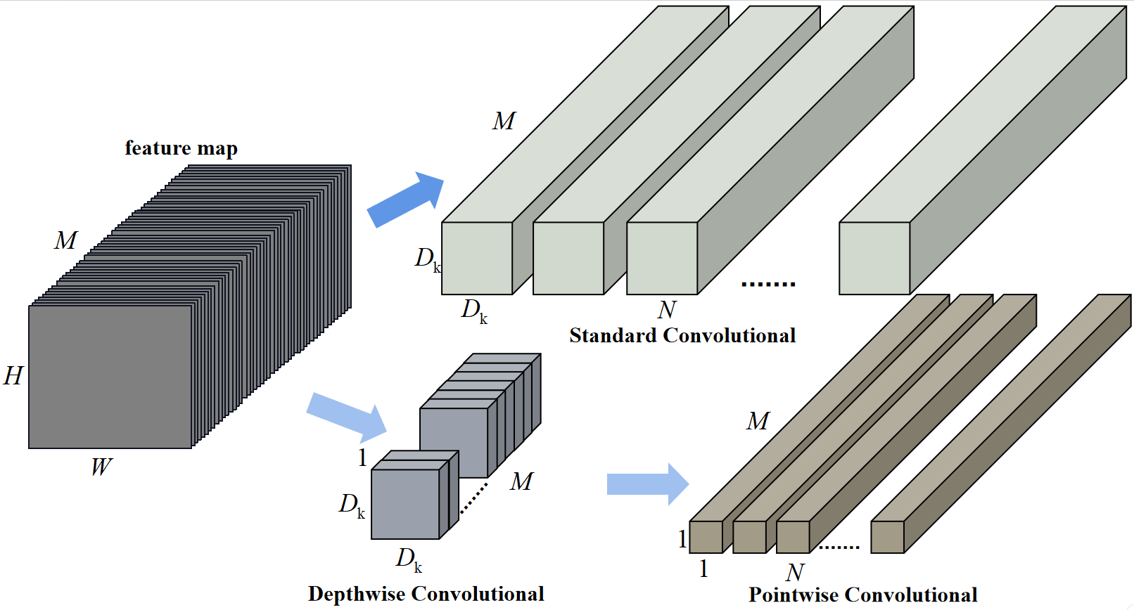
每个独立长方体表示一个卷积核，长方体的长度就表示卷积核的通道数。

普通卷积：输入是M个通道，输出是N个通道；
深度可分离卷积：深度卷积输入是1个通道，输出是M个通道；点卷积输入是M个通道，输出是N个通道。

普通卷积

为了方便比较俩者在卷积过程中的差异，本小节回过一下普通卷积的卷积过程，如下图所示：

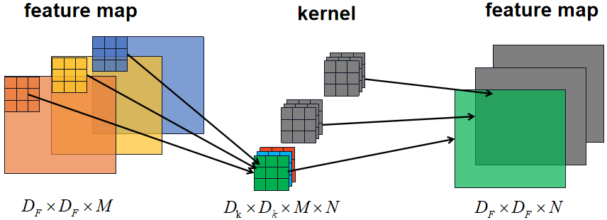
普通卷积的参数量： ${D_K} \times {D_K}\times M \times N$
普通卷积的计算量： ${D_F} \times {D_F} \times M \times N \times {D_K} \times {D_K}$

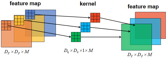
Depthwise Convolutional(深度卷积)

深度卷积对于输入特征图的每个通道单独应用一个卷积核进行卷积，卷积的输入通道则是1，输入特征图有M个通道则需要M个卷积核，输出通道则是M：

深度卷积的参数量： ${D_K} \times {D_K}\times 1 \times M$
深度卷积的计算量： ${D_F} \times {D_F} \times 1 \times M \times {D_K} \times {D_K}$

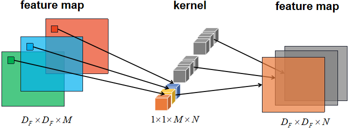
Pointwise Convolution(点卷积)

应用普通的1×1卷积层将深度卷积后输出的特征图的所有通道信息进行整合，1×1卷积的输入通道是M，输出通道是N：

点卷积的参数量： $\times 1 \times M \times N$
点卷积的计算量： ${D_F} \times {D_F} \times M \times N \times 1 \times 1$

普通卷积和深度可分离卷积的比较

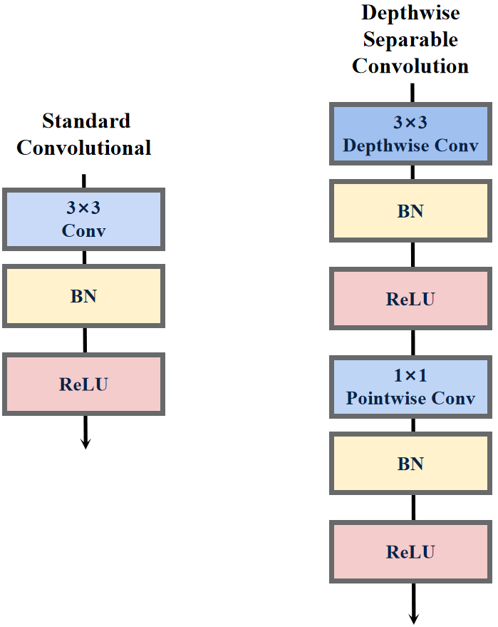
结构对比：普通卷积包括3×3卷积层+BN层+激活函数；深度可分离卷积包括3×3深度卷积层+BN层+激活函数和1×1点卷积层+BN层+激活函数。
参数量对比：
$\frac{{1 \times M \times {D_K} \times {D_K} + M{\rm{ \times }}N \times 1 \times 1}}{{M \times N \times {D_K} \times {D_K}}} = \frac{1}{N} + \frac{1}{{D_K^2}}$
计算量对比：
$\frac{{{D_F} \times {D_F} \times 1 \times M \times {D_K} \times {D_K} + {D_F} \times {D_F} \times M{\rm{ \times }}N \times 1 \times 1}}{{{D_F} \times {D_F} \times M \times N \times {D_K} \times {D_K}}} = \frac{1}{N} + \frac{1}{{D_K^2}}$
对比乘法运算次数，深度可分离卷积虽然分为两部分，但计算速度更快，理论上普通卷积计算量是深度可分离卷积的8到9倍(因为卷积核通常是3×3)

各位读者要仔细分清每个字母代表的含义

MobleNet_V1模型结构

下图是原论文给出的关于MobileNets_V1模型结构的详细示意图：

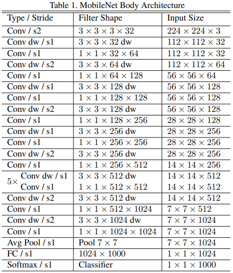
MobileNets_V1在图像分类中分为两部分：backbone部分： 主要由普通卷积层、深度可分离卷积层组成，分类器部分：由池化层(汇聚层)和全连接层组成。
MobileNets_V1除了第一层是普通卷积层外，其他都是深度可分离卷积层。除了全连接层没有ReLU层外，每个网络层后都有BN层和ReLU非线性激活层，全连接层最后接softmax层进行分类。

超参数	功能
α	控制模型中所有层的输入输出通道： K×K×M×1+1×1×M×N⇒K×K×αM×1+αM×αN
ρ	减少网络输入图像的分辨率：(K×K×M×1+1×1×M×N)×F×F⇒(K×K×M+×M×N)×ρF×ρF

MobleNet_V1 Pytorch代码

普通卷积块： 3×3卷积层+BN层+LeakyReLU激活函数

# 普通卷积块
def conv_bn(inp, oup, stride = 1, leaky = 0.1):
    return nn.Sequential(
        nn.Conv2d(inp, oup, 3, stride, 1, bias=False),
        nn.BatchNorm2d(oup),
        nn.LeakyReLU(negative_slope=leaky, inplace=True)
    )

深度可分离卷积块： 3×3深度卷积层+BN层+LeakyReLU激活函数+1×1点卷积层+BN层+LeakyReLU激活函数

# 深度可分离卷积块
def conv_dw(inp, oup, stride = 1, leaky=0.1):
    return nn.Sequential(
        nn.Conv2d(inp, inp, 3, stride, 1, groups=inp, bias=False),
        nn.BatchNorm2d(inp),
        nn.LeakyReLU(negative_slope=leaky, inplace=True),

        nn.Conv2d(inp, oup, 1, 1, 0, bias=False),
        nn.BatchNorm2d(oup),
        nn.LeakyReLU(negative_slope=leaky, inplace=True),
    )

这里有必要说明一下Convolution层中的group参数，其意思是将对应的输入通道与输出通道数进行分组, 默认值为1(普通卷积), 即输出输入的所有通道各为一组。假设group是2，那么对应要将输入的32个通道分成2个16的通道，将输出的48个通道分成2个24的通道。对输出的2个24的通道，第一个24通道与输入的第一个16通道进行全卷积，第二个24通道与输入的第二个16通道进行全卷积。这里只需要记住，MobileNets_V1的group数与输入特征图的通道数一致。

完整代码

import torch.nn as nn
import torch
from torchsummary import summary

def _make_divisible(ch, divisor=8, min_ch=None):
    if min_ch is None:
        min_ch = divisor
    '''
    int(ch + divisor / 2) // divisor * divisor)
    目的是为了让new_ch是divisor的整数倍
    类似于四舍五入:ch超过divisor的一半则加1保留;不满一半则归零舍弃
    '''
    new_ch = max(min_ch, int(ch + divisor / 2) // divisor * divisor)
    # 假设new_ch小于ch的0.9倍,则再加divisor
    if new_ch < 0.9 * ch:
        new_ch += divisor
    return new_ch

# 普通卷积块
def conv_bn(inp, oup, stride = 1, leaky = 0.1):
    return nn.Sequential(
        nn.Conv2d(inp, oup, 3, stride, 1, bias=False),
        nn.BatchNorm2d(oup),
        nn.LeakyReLU(negative_slope=leaky, inplace=True)
    )
# 深度可分离卷积块
def conv_dw(inp, oup, stride = 1, leaky=0.1):
    return nn.Sequential(
        nn.Conv2d(inp, inp, 3, stride, 1, groups=inp, bias=False),
        nn.BatchNorm2d(inp),
        nn.LeakyReLU(negative_slope=leaky, inplace=True),

        nn.Conv2d(inp, oup, 1, 1, 0, bias=False),
        nn.BatchNorm2d(oup),
        nn.LeakyReLU(negative_slope=leaky, inplace=True),
    )
class MobileNetV1(nn.Module):
    def __init__(self, alpha, round_nearest=8):
        super(MobileNetV1, self).__init__()
        self.stage1 = nn.Sequential(
            conv_bn(3, _make_divisible(32*alpha, round_nearest), 2, leaky=0.1),
            conv_dw(_make_divisible(32*alpha, round_nearest), _make_divisible(64*alpha, round_nearest), 1),
            conv_dw(_make_divisible(64*alpha, round_nearest), _make_divisible(128*alpha, round_nearest), 2),
            conv_dw(_make_divisible(128*alpha, round_nearest), _make_divisible(128*alpha, round_nearest), 1),
            conv_dw(_make_divisible(128*alpha, round_nearest), _make_divisible(256*alpha, round_nearest), 2),
            conv_dw(_make_divisible(256*alpha, round_nearest), _make_divisible(256*alpha, round_nearest), 1),
        )
        self.stage2 = nn.Sequential(
            conv_dw(_make_divisible(256*alpha, round_nearest), _make_divisible(512*alpha, round_nearest), 2),
            conv_dw(_make_divisible(512*alpha, round_nearest), _make_divisible(512*alpha, round_nearest), 1),
            conv_dw(_make_divisible(512*alpha, round_nearest), _make_divisible(512*alpha, round_nearest), 1),
            conv_dw(_make_divisible(512*alpha, round_nearest), _make_divisible(512*alpha, round_nearest), 1),
            conv_dw(_make_divisible(512*alpha, round_nearest), _make_divisible(512*alpha, round_nearest), 1),
            conv_dw(_make_divisible(512*alpha, round_nearest), _make_divisible(512*alpha, round_nearest), 1),
        )
        self.stage3 = nn.Sequential(
            conv_dw(_make_divisible(512*alpha, round_nearest), _make_divisible(1024*alpha, round_nearest), 2),
            conv_dw(_make_divisible(1024*alpha, round_nearest), _make_divisible(1024*alpha, round_nearest), 1),
        )
        self.avg = nn.AdaptiveAvgPool2d((1, 1))
        self.fc = nn.Linear(_make_divisible(1024*alpha, round_nearest), 1000)

    def forward(self, x):
        # mobilenetV1 0.25为例
        # N x 3 x 224 x 224
        x = self.stage1( x )
        # N x 64 x 28 x 28
        x = self.stage2( x )
        # N x 128 x 14 x 14
        x = self.stage3( x )
        # N x 256 x 7 x 7
        x = self.avg( x )
        # N x 256 x 1 x 1
        x = x.view(-1,256)
        # N x 256
        x = self.fc(x)
        # N x 1000
        return x
        
# mobilenetV1 0.25
def MobileNetV1x25():
    return MobileNetV1(alpha=0.25)

# mobilenetV1 0.50
def MobileNetV1x50():
    return MobileNetV1(alpha=0.5, round_nearest=8)

# mobilenetV1 0.75
def MobileNetV1x75():
    return MobileNetV1(alpha=0.75, round_nearest=8)

# mobilenetV1 1.00
def MobileNetV1x100():
    return MobileNetV1(alpha=1.0, round_nearest=8)

if __name__ == '__main__':
    device = torch.device("cuda:0" if torch.cuda.is_available() else "cpu")
    model = MobileNetV1x25().to(device)
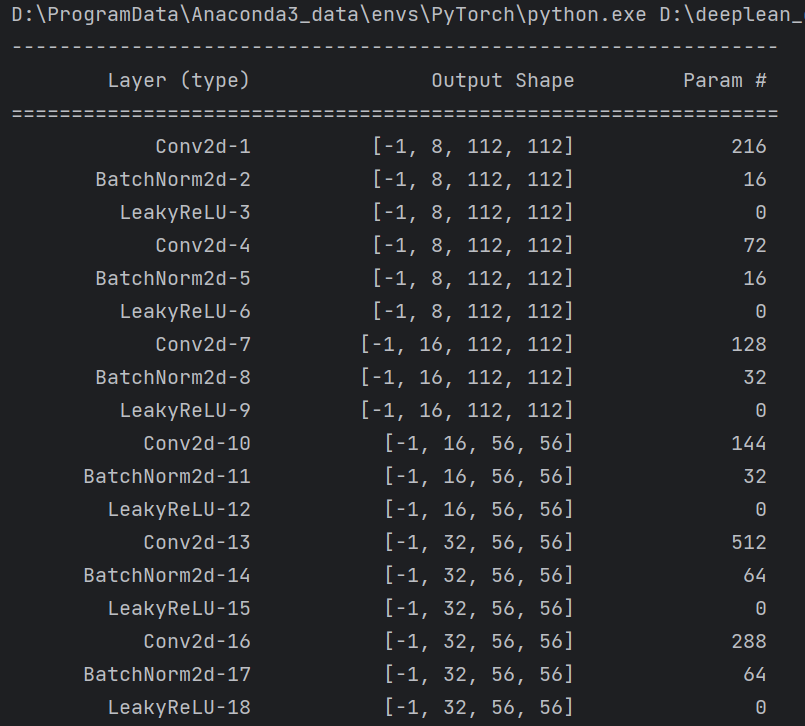
    summary(model, input_size=(3, 224, 224))