


书生·浦语训练营:第五讲 LmDeploy 量化部署
参考资料:
zeux.io - LLM inference speed of light
https://github.com/InternLM/Tutorial/tree/camp2/lmdeploy
[译] 大模型推理的极限:理论分析、数学建模与 CPU/GPU 实测(2024)
0 推理机制
0.1 transformer逐个生成token
当语言模型生成文本时,它是逐个 token 进行的,无法并行处理。
- 输入:一个 token
- 输出:一组概率,每个概率对应词汇表中一个 token。
- 推理程序使用概率来指导抽样,产生(从词汇表中选择)下一个 token 作为最终输出。
0.2 生成过程建模:矩阵乘法
广义上,当处理一个 token 时,模型执行两种类型的操作:
-
矩阵-向量乘法:一个大矩阵(例如 8192x8192)乘以一个向量,得到另一个向量,
-
attention 计算。
在生成过程中,模型不仅可以看到当前 token 的状态,还可以看到序列中所有之前 token 的内部状态 —— 这些状态被存储在一个称为
KV-cache的结构中, 它本质上是文本中每个之前位置的 key 向量和 value 向量的集合。attention 为当前 token 生成一个 query 向量,计算它与所有之前位置的 key 向量之间的点积, 然后归一化得到的一组标量,并通过对所有之前的 value 向量进行加权求和来计算一个 value 向量,使用点积得到最终得分。
0.3 什么是KV-cache?
生成式模型的推断流程是将当前轮输出 token 与之前轮次的输入tokens拼接,并作为下一轮的输入tokens,反复多次。可以看出第 i+1 轮输入数据只比第 i 轮输入数据新增了一个 token,其他全部相同。因此第 i+1 轮推理时必然包含了第 i 轮的部分计算。KV Cache的出发点就是缓存当前轮可重复利用的计算结果,下一轮计算时直接读取缓存结果。在自回归编码的过程中Q值用完就可以丢弃,无需缓存Q。
对于 Mistral,KV-cache
- 为每层的每个 key 存储 8 个 128 元素向量,
- 为每个层的每个 value 存储 8 个 128 元素向量,
加起来,每个 token 对应 32 * 128 * 8 * 2 = 65K 个元素; 如果 KV-cache 使用 FP16,那么对于 token number P,我们需要读取 P * 130 KB 的数据。 例如, token number 1000 将需要从 KV-cache 读取 130MB 的数据。 跟 14.2GB 这个总数据量相比,这 130MB 可以忽略不计了。
1 定义
在软件工程中,部署通常指将开发完的软件投入使用的过程。在人工智能领域,模型部署是实现实现深度学习算法落地的关键步骤。简单来说,模型部署就是将训好的深度学习模型在特定环境中运行的过程。
2 大模型部署遇到的挑战
2.1 计算量巨大
| Operation | Parameters | FLOPs per Token |
|---|---|---|
| Embed | ( n v o c a b + n c t x ) d m o d e l (n_{vocab} + n_{ctx})d_{model} (nvocab+nctx)dmodel | 4 d m o d e l 4d_{model} 4dmodel |
| Attention: QKV | n l a y e r d m o d e l 3 d a t t n n_{layer}d_{model}3d_{attn} nlayerdmodel3dattn | 2 n l a y e r d m o d e l 3 d a t t n 2n_{layer}d_{model}3d_{attn} 2nlayerdmodel3dattn |
| Attention: Mask | —— | 2 n l a y e r n c t x d a t t n 2n_{layer}n_{ctx}d_{attn} 2nlayernctxdattn |
| Attention: Project | n l a y e r d m o d e l d a t t n n_{layer}d_{model}d_{attn} nlayerdmodeldattn | 2 n l a y e r d a t t n d e m b d 2n_{layer}d_{attn}d_{embd} 2nlayerdattndembd |
| Feedforward | n l a y e r 2 d m o d e l d f f n_{layer}2d_{model}d_{ff} nlayer2dmodeldff | 2 n l a y e r 2 d m o d e l d f f 2n_{layer}2d_{model}d_{ff} 2nlayer2dmodeldff |
| De-embed | —— | 2 d m o d e l x n v o c a b 2d_{modelx}n_{vocab} 2dmodelxnvocab |
| Total (Non-Embedding) | N = 2 d m o d e l n l a y e r ( 2 d a t t n + d f f ) N=2d_{model}n_{layer}(2d_{attn}+d_{ff}) N=2dmodelnlayer(2dattn+dff) | C f o r w a r d = 2 N + 2 n l a y e r n c t x d a t t n C_{forward}=2N+2n_{layer}n_{ctx}d_{attn} Cforward=2N+2nlayernctxdattn |
其中,N为模型参数量, n l a y e r n_{layer} nlayer为模型层数, n c t x n_{ctx} nctx为上下文长度(默认1024) d a t t n d_{attn} dattn为注意力输出维度, d f f d_{ff} dff表示前馈网络隐藏层维度。
表格中的数据还是蛮好理解的,注意力层的QKV三个矩阵对应了三个线性层,映射层对应了一个线性层,前馈网络里面包含了2个线性层。
Flop表示浮点数运算次数,衡量了计算量的大小。对于 A ∈ R 1 × n , B ∈ R n × 1 A\in R^{1\times n},B\in R^{n \times 1} A∈R1×n,B∈Rn×1,计算
A B AB AB 点积需要进行 n 次乘法运算和 n 次加法运算,共计 2n 次浮点数运算,需要 2n 的FLOPs。对于 A ∈ R m × n , B ∈ R n × p A\in R^{m\times n},B\in R^{n \times p} A∈Rm×n,B∈Rn×p ,计算 A B AB AB 需要的浮点数运算次数为 2mnp。
20B模型每生成1个token,就要进行406亿次浮点运算,若生成128个token,就要进行5.2万亿次运算。若参数规模达到175B(GPT-3)每次推理计算量将达到千万亿量级。
以NVIDIA A100为例,单张理论FP16运算性能为77.97 TFLOPs(77万亿)。
以internLM2的1.8B、7B、20B模型为例,计算量估算为:
| N | n l a y e r n_{layer} nlayer | d a t t n d_attn dattn | C f o r w a w r d C_{forwawrd} Cforwawrd |
|---|---|---|---|
| 1.8 B | 24 | 2048 | 3.7 GFLOPs |
| 7 B | 32 | 4096 | 14.2 GFLOPs |
| 20 B | 48 | 6144 | 40.6 GFLOPs |
2.2 访存瓶颈
大模型推理是“访存密集”型任务。目前硬件计算速度“远快于”显存带宽,因此实际部署大模型时不能仅仅考虑计算量,还应该考虑访存的瓶颈。
以 RTX 4090推理175B大模型为例,BS为1时计算量为6.83 TFLOPs,远低于82.58 TFLOPs的FP16计算能力;但访存量为32.62TB,是显存带宽每秒处理能力30倍。说明即使GPU很快完成计算也需要等待漫长的数据交换。
2.3 动态请求
- 请求量不确定
- 请求时间不确定
- Token逐个生成,生成数量不确定
3 解决方案
3.1 模型剪枝
大模型的参数量极为庞大,研究发现并不是所有的参数都会发挥作用,因此可以对模型进行剪枝处理,移除模型不必要的组件,从而使模型更加高效。通过对模型中贡献有限的冗余参数进行剪枝,在保证性能最低下降的同时,可以减小存储需求,提高计算效率。
非结构化剪枝:SparseGPT、LoRAPrune、Wanda
移除个别参数,不考虑整体网络结构
结构化剪枝:LLM-Pruner
根据预定义规则移除连接或分层结构,同时保持整体网络结构。
3.2 知识蒸馏
知识蒸馏是一种经典的模型压缩方法,往往训练一个参数量较小的模型却希望他能够达到较好的效果是很困难的,知识蒸馏通过引导轻量化学生模型“模仿”性能更好、结构更复杂的教师模型,在不改变学生模型结构的情况下提高其性能。
3.3 量化
量化技术是将传统表示方法中的浮点数转换为整数或其他离散的形式。模型往往以32为浮点数存储参数,但往往不需要这么高的精度,因此可以通过量化的方式损失一点模型的精度,却不怎么影响模型的性能,从而减少了数据传输所需要的时间,减少了计算负担。
4 Lmdeploy部署
4.1 Lmdeploy环境配置
step 1.创建开发机
step 2.配置conda环境
conda create -n lmdeploy -y python=3.10
conda activate lmdeploy
# 安装0.3.0的lmdeploy
pip install lmdeploy[all]==0.3.0
4.2 利用InternStudio下载模型
ls /root/share/new_models/Shanghai_AI_Laboratory/
4.3 使用Lmdeploy部署模型对话
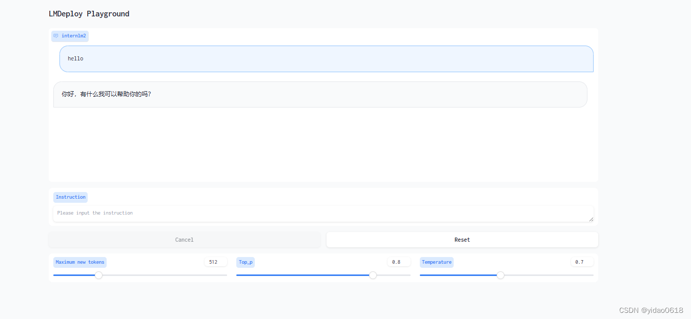
(输入你的问题并且按两下回车,输入exit按下两次回车退出)
lmdeploy chat /root/internlm2-chat-1_8b
4.3 使用Lmdeploy进行模型量化
前文提到decoder-only属于访存密集型,大部分时间都浪费在数据交换上。如何优化 LLM 模型推理中的访存密集问题呢? 我们可以使用KV8量化和W4A16量化。KV8量化是指将逐 Token(Decoding)生成过程中的上下文 K 和 V 中间结果进行 INT8 量化(计算时再反量化),以降低生成过程中的显存占用。W4A16 量化,将 FP16 的模型权重量化为 INT4,Kernel 计算时,访存量直接降为 FP16 模型的 1/4,大幅降低了访存成本。Weight Only 是指仅量化权重,数值计算依然采用 FP16(需要将 INT4 权重反量化)。
KV Cache是一种缓存技术,通过存储键值对的形式来复用计算结果,以达到提高性能和降低内存消耗的目的。在大规模训练和推理中,KV Cache可以显著减少重复计算量,从而提升模型的推理速度。理想情况下,KV Cache全部存储于显存,以加快访存速度。当显存空间不足时,也可以将KV Cache放在内存,通过缓存管理器控制将当前需要使用的数据放入显存。
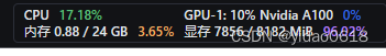
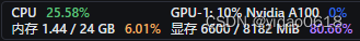
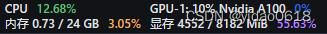
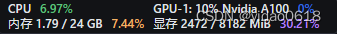
模型在运行时,占用的显存可大致分为三部分:模型参数本身占用的显存、KV Cache占用的显存,以及中间运算结果占用的显存。LMDeploy的KV Cache管理器可以通过设置--cache-max-entry-count参数,控制KV缓存占用剩余显存的最大比例。默认的比例为0.8。
# --cache-max-entry-count的默认值为0.8
lmdeploy chat /root/internlm2-chat-1_8b
# 设置--cache-max-entry-count为0.5
lmdeploy chat /root/internlm2-chat-1_8b --cache-max-entry-count 0.5
# 设置--cache-max-entry-count为0.01,代价是会降低推理速度
lmdeploy chat /root/internlm2-chat-1_8b --cache-max-entry-count 0.01
LMDeploy使用AWQ算法,实现模型4bit权重量化。推理引擎TurboMind提供了非常高效的4bit推理cuda kernel,性能是FP16的2.4倍以上。
# 安装相关依赖
pip install einops==0.7.0
# 进行模型量化
lmdeploy lite auto_awq \
   /root/internlm2-chat-1_8b \
  --calib-dataset 'ptb' \
  --calib-samples 128 \
  --calib-seqlen 1024 \
  --w-bits 4 \
  --w-group-size 128 \
  --work-dir /root/internlm2-chat-1_8b-4bit
# 运行量化后的模型
lmdeploy chat /root/internlm2-chat-1_8b-4bit --model-format awq
# 设置KV-cache并运行量化后的模型
lmdeploy chat /root/internlm2-chat-1_8b-4bit --model-format awq --cache-max-entry-count 0.01
4.4 模型部署
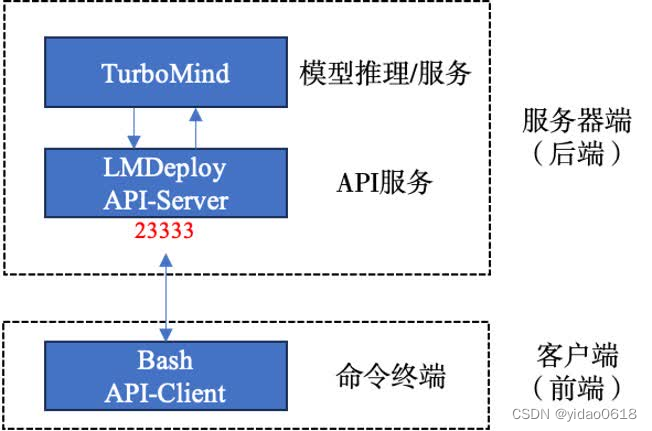
4.4.1 利用API Sever
# 启动API Sever
lmdeploy serve api_server \
    /root/internlm2-chat-1_8b \
    --model-format hf \
    --quant-policy 0 \
    --server-name 0.0.0.0 \
    --server-port 23333 \
    --tp 1
在InternStudio中通过VS Code新建终端
conda activate lmdeploy
lmdeploy serve api_client http://localhost:23333
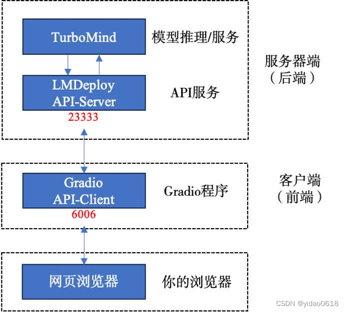
4.4.2 通过网页客户端
# 使用gradio作为前端
lmdeploy serve gradio http://localhost:23333 \
    --server-name 0.0.0.0 \
    --server-port 6006
本地使用PowerShell
ssh -CNg -L 6006:127.0.0.1:6006 root@ssh.intern-ai.org.cn -p <你的ssh端口号>
4.4.3 Python代码集成
# 返回InternStudio在root目录下新建文件pipeline.py
touch /root/pipeline.py
pipeline.py填入下面内容:
from lmdeploy import pipeline, TurbomindEngineConfig

# 调低 k/v cache内存占比调整为总显存的 20%
backend_config = TurbomindEngineConfig(cache_max_entry_count=0.2)

pipe = pipeline('/root/internlm2-chat-1_8b',
                backend_config=backend_config)  # 连接大模型,并设置kv cache总显存占比
response = pipe(['Hi, pls intro yourself', '上海是'])  # 提问列表中的内容,返回response
print(response)
4.4.4 使用Lmdeploy运行多模态大模型llava
conda activate lmdeploy
# 安装依赖
pip install git+https://github.com/haotian-liu/LLaVA.git@4e2277a060da264c4f21b364c867cc622c945874
# 新建python文件
touch /root/pipeline_llava.py
在pipeline_llava.py写入:
from lmdeploy.vl import load_image
from lmdeploy import pipeline, TurbomindEngineConfig


backend_config = TurbomindEngineConfig(session_len=8192) # 图片分辨率较高时请调高session_len
# pipe = pipeline('liuhaotian/llava-v1.6-vicuna-7b', backend_config=backend_config) 非开发机运行此命令
pipe = pipeline('/share/new_models/liuhaotian/llava-v1.6-vicuna-7b', backend_config=backend_config)  # 加载模型

image = load_image('https://raw.githubusercontent.com/open-mmlab/mmdeploy/main/tests/data/tiger.jpeg')  # 加载链接中图片,可以替换成本地图片
response = pipe(('describe this image', image))  # 传入llava
print(response)
我们也可以通过Gradio来运行llava模型。新建python文件gradio_llava.py。
touch /root/gradio_llava.py
在gradio_llava.py中写入:
import gradio as gr
from lmdeploy import pipeline, TurbomindEngineConfig


backend_config = TurbomindEngineConfig(session_len=8192) # 图片分辨率较高时请调高session_len
# pipe = pipeline('liuhaotian/llava-v1.6-vicuna-7b', backend_config=backend_config) 非开发机运行此命令
pipe = pipeline('/share/new_models/liuhaotian/llava-v1.6-vicuna-7b', backend_config=backend_config)

def model(image, text):
    if image is None:
        return [(text, "请上传一张图片。")]
    else:
        response = pipe((text, image)).text
        return [(text, response)]

demo = gr.Interface(fn=model, inputs=[gr.Image(type="pil"), gr.Textbox()], outputs=gr.Chatbot())
demo.launch()
使用PowerShell
ssh -CNg -L 7860:127.0.0.1:7860 root@ssh.intern-ai.org.cn -p <你的ssh端口>
5 定量比较LMDeploy与Transformer库的推理速度差异
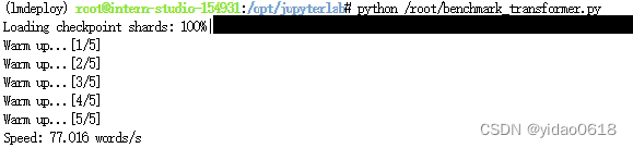
新建benchmark_transformer.py
在benchmark_transformer.py写入:
import torch
import datetime
from transformers import AutoTokenizer, AutoModelForCausalLM

tokenizer = AutoTokenizer.from_pretrained("/root/internlm2-chat-1_8b", trust_remote_code=True)

# Set `torch_dtype=torch.float16` to load model in float16, otherwise it will be loaded as float32 and cause OOM Error.
model = AutoModelForCausalLM.from_pretrained("/root/internlm2-chat-1_8b", torch_dtype=torch.float16, trust_remote_code=True).cuda()
model = model.eval()

# warmup
inp = "hello"
for i in range(5):
    print("Warm up...[{}/5]".format(i+1))
    response, history = model.chat(tokenizer, inp, history=[])

# test speed
inp = "请介绍一下你自己。"
times = 10
total_words = 0
start_time = datetime.datetime.now()
for i in range(times):
    response, history = model.chat(tokenizer, inp, history=history)
    total_words += len(response)
end_time = datetime.datetime.now()

delta_time = end_time - start_time
delta_time = delta_time.seconds + delta_time.microseconds / 1000000.0
speed = total_words / delta_time
print("Speed: {:.3f} words/s".format(speed))
新建benchmark_lmdeploy.py,并填入以下内容:
import datetime
from lmdeploy import pipeline

pipe = pipeline('/root/internlm2-chat-1_8b')

# warmup
inp = "hello"
for i in range(5):
    print("Warm up...[{}/5]".format(i+1))
    response = pipe([inp])

# test speed
inp = "请介绍一下你自己。"
times = 10
total_words = 0
start_time = datetime.datetime.now()
for i in range(times):
    response = pipe([inp])
    total_words += len(response[0].text)
end_time = datetime.datetime.now()

delta_time = end_time - start_time
delta_time = delta_time.seconds + delta_time.microseconds / 1000000.0
speed = total_words / delta_time
print("Speed: {:.3f} words/s".format(speed))
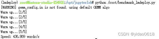
可以看到速度提升了将近6倍。


 1878
1878


 被折叠的 条评论
为什么被折叠?
被折叠的 条评论
为什么被折叠?
 到【灌水乐园】发言


