


 本文介绍了如何使用MATLAB的SignalProcessingToolbox生成周期性和非周期性波形,包括锯齿波、方波、三角脉冲、矩形脉冲、高斯脉冲、扫频波形和脉冲序列。示例代码展示了函数如sawtooth、square、chirp和pulstran的用法,以及diric函数计算Dirichlet函数。
信号生成和可视化——周期性/非周期性波形
目录
tripuls、rectpuls 和 gauspuls 函数
gauspuls 函数使用指定时间、中心频率和小数带宽生成高斯调制正弦脉冲。
此示例说明如何使用 Signal Processing Toolbox™ 中提供的函数生成广泛使用的周期和非周期性波形、扫频正弦波和脉冲序列。尝试此示例Copy Command Copy Code
周期性波形
除了 MATLAB® 中的 sin 和 cos 函数外,Signal Processing Toolbox™ 还提供其他函数(如 sawtooth 和 square)来生成周期性信号。
sawtooth 函数生成锯齿波
sawtooth 函数生成锯齿波,波峰在 ±1,周期为 2π。可选宽度参数以 2π 的小数倍来指定信号最大值出现的位置。
square 函数生成方波
square 函数生成周期为 2π 的方波。可选参数指定占空比,即信号为正的周期的百分比。
% % 以 10 kHz 的采样率生成 1.5 秒的 50 Hz 锯齿波。对一个方波进行重复计算。
fs = 10000; %以10kHz的采样率
t = 0:1/fs:1.5;
x1 = sawtooth(2*pi*50*t); %锯齿波
x2 = square(2*pi*50*t); %方波

subplot(2,1,1) % subplot(m,n,p) 将当前图窗划分为 m×n 网格,并在 p 指定的位置创建坐标区。
plot(t,x1)%二维线图
axis([0 0.2 -1.2 1.2])%设置坐标轴范围x[0,0.2], y[-1.2,1.2]
xlabel('Time (sec)')
ylabel('Amplitude')
title('Sawtooth Periodic Wave')

subplot(2,1,2)
plot(t,x2)
axis([0 0.2 -1.2 1.2])
xlabel('Time (sec)')
ylabel('Amplitude')
title('Square Periodic Wave')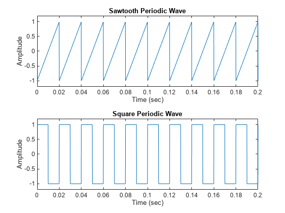
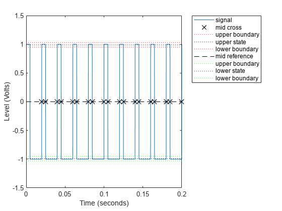
% 使用 dutycycle 函数验证方波的占空比是否为指定值。
% 不带输出参数调用该函数来绘制波形、中间参考瞬时电平的位置、相关联的参考电平、状态电平以及相关联的状态上下边界。
figure
dc = dutycycle(x2,fs);
dc = dc(1);
% disp(dc);%输出dc的值
fprintf('the value of dc is%6.2f\n',dc)%输出dc的值
dutycycle(x2,fs);
xlim([0 0.2])
非周期性波形
tripuls、rectpuls 和 gauspuls 函数
为了生成三角形、矩形和高斯脉冲,工具箱提供了 tripuls、rectpuls 和 gauspuls 函数。
tripuls 函数生成以 t = 0 为中心、默认宽度为 1 的采样非周期性单位高度三角形脉冲。
rectpuls 函数生成以 t = 0 为中心、默认宽度为 1 的采样非周期性单位高度矩形脉冲。非零幅值的区间定义为在右侧开放:rectpuls(-0.5) = 1,而 rectpuls(0.5) = 0。
% % 生成 2 秒的三角形脉冲,采样率为 10 kHz,宽度为 20 ms。对一个矩形脉冲进行重复计算。
fs = 10000;
t = -1:1/fs:1;
x1 = tripuls(t,20e-3);
x2 = rectpuls(t,20e-3);

figure
subplot(2,1,1)
plot(t,x1)
axis([-0.1 0.1 -0.2 1.2])
xlabel('Time (sec)')
ylabel('Amplitude')
title('Triangular Aperiodic Pulse')

subplot(2,1,2)
plot(t,x2)
axis([-0.1 0.1 -0.2 1.2])
xlabel('Time (sec)')
ylabel('Amplitude')
title('Rectangular Aperiodic Pulse')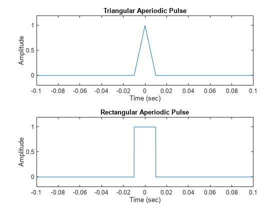
gauspuls 函数使用指定时间、中心频率和小数带宽生成高斯调制正弦脉冲。
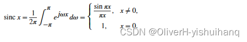
sinc 函数计算输入向量或矩阵的数学正弦函数
sinc 函数计算输入向量或矩阵 x 的数学正弦函数。作为时间或空间的函数,sinc 函数是以零为中心、宽度为 2π 并具有单位高度的频率的矩形脉冲的傅里叶逆变换:
% 生成带宽为 60%、采样率为 1 MHz 的 50 kHz 高斯 RF 脉冲。
% 当包络比峰值低 40 dB 时,截断脉冲。
tc = gauspuls('cutoff',50e3,0.6,[],-40);
t1 = -tc : 1e-6 : tc;
y1 = gauspuls(t1,50e3,0.6);
% 为一个线性间距向量生成正弦函数:
t2 = linspace(-5,5);
y2 = sinc(t2);

figure
subplot(2,1,1)
plot(t1*1e3,y1)
xlabel('Time (ms)')
ylabel('Amplitude')
title('Gaussian Pulse')

subplot(2,1,2)
plot(t2,y2)
xlabel('Time (sec)')
ylabel('Amplitude')
title('Sinc Function')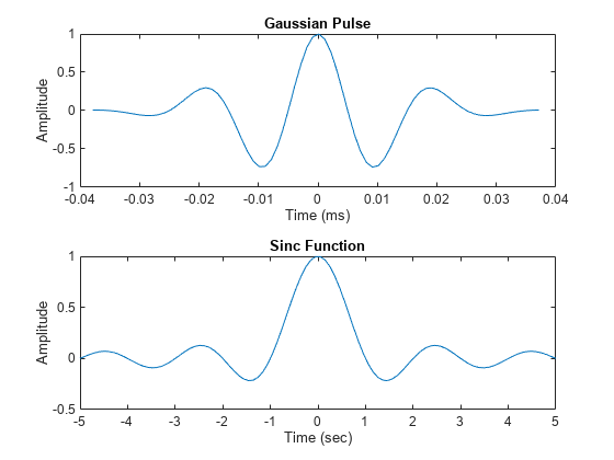
扫频波形
chirp 函数生成线性或二次、凸和凹二次 chirp
工具箱还提供生成扫频波形的函数,如 chirp 函数。两个可选参数以度为单位指定替代扫描方法和初始相位。
chirp 生成线性、对数或二次扫频正弦信号。可选参数指定替代扫描方法。可选参数允许以度数指定初始相位。
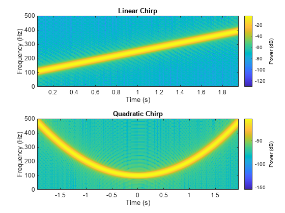
下面是使用 chirp 函数生成线性或二次、凸和凹二次 chirp 的几个示例。
% 生成线性 chirp。

t = 0:0.001:2; % 2 secs @ 1kHz sample rate

ylin = chirp(t,0,1,150); % Start @ DC, cross 150Hz at t=1sec
% 绘制 chirp 的频谱图。指定相邻窗段之间的重叠为 90%。

figure
pspectrum(ylin,t,'spectrogram','OverlapPercent',90)


% 生成二次 chirp。

t = -2:0.001:2; % +/-2 secs @ 1kHz sample rate

yq = chirp(t,100,1,200,'q'); % Start @ 100Hz, cross 200Hz at t=1sec

% 计算并显示 chirp 的频谱图。

figure

subplot(2,1,1)

spectrogram(ylin,256,250,256,1E3,'yaxis')

title('Linear Chirp')

subplot(2,1,2)

spectrogram(yq,128,120,128,1E3,'yaxis')

title('Quadratic Chirp')
% 生成凸二次 chirp。

t = -1:0.001:1; % +/-1 second @ 1kHz sample rate

fo = 100;

f1 = 400; % Start at 100Hz, go up to 400Hz

ycx = chirp(t,fo,1,f1,'q',[],'convex');

% 生成凹二次 chirp。

t = -1:0.001:1; % +/-1 second @ 1kHz sample rate

fo = 400;

f1 = 100; % Start at 400Hz, go down to 100Hz

ycv = chirp(t,fo,1,f1,'q',[],'concave');

% 计算并显示 chirp 的频谱图。

figure

subplot(2,1,1)

spectrogram(ycx,256,255,128,1000,'yaxis')

title('Convex Chirp')

subplot(2,1,2)

spectrogram(ycv,256,255,128,1000,'yaxis')

title('Concave Chirp')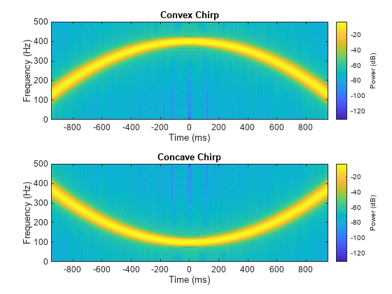
另一个函数生成器是 vco(压控振荡器),它生成以输入向量确定的频率振荡的信号。输入向量可以是三角形、矩形或正弦波等。
% 生成以 10 kHz 采样的 2 秒信号,其瞬时频率为三角形。对一个矩形进行重复计算。
fs = 10000;
t = 0:1/fs:2;
x1 = vco(sawtooth(2*pi*t,0.75),[0.1 0.4]*fs,fs);
x2 = vco(square(2*pi*t),[0.1 0.4]*fs,fs);

% 绘制生成的信号的频谱图。
figure
subplot(2,1,1)
spectrogram(x1,kaiser(256,5),220,512,fs,'yaxis')
title('VCO Triangle')

subplot(2,1,2)
spectrogram(x2,256,255,256,fs,'yaxis')
title('VCO Rectangle')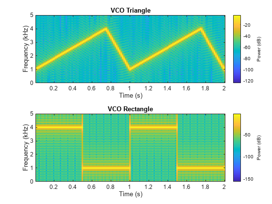
脉冲序列
pulstran 函数生成脉冲序列波
要生成脉冲序列,您可以使用 pulstran 函数。
% 构造一个 2 GHz 矩形脉冲序列,它以 7.5 ns 的间距和 100 GHz 的速率采样。
fs = 100E9;                    % sample freq
D = [2.5 10 17.5]' * 1e-9;     % pulse delay times
t = 0 : 1/fs : 2500/fs;        % signal evaluation time
w = 1e-9;                      % width of each pulse
yp = pulstran(t,D,@rectpuls,w);

% 生成 10 kHz、50% 带宽的周期性高斯脉冲信号。脉冲重复频率为 1 kHz,采样率为 50 kHz,
% 脉冲序列长度为 10 毫秒。重复幅值每次应按 0.8 衰减。
% 使用函数句柄指定生成器函数。
T = 0 : 1/50e3 : 10e-3;
D = [0 : 1/1e3 : 10e-3 ; 0.8.^(0:10)]';
Y = pulstran(T,D,@gauspuls,10E3,.5);

figure
subplot(2,1,1)
plot(t*1e9,yp);
axis([0 25 -0.2 1.2])
xlabel('Time (ns)')
ylabel('Amplitude')
title('Rectangular Train')

subplot(2,1,2)
plot(T*1e3,Y)
xlabel('Time (ms)')
ylabel('Amplitude')
title('Gaussian Pulse Train')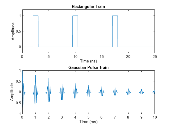
Dirichlet 函数
diric 函数计算输入向量或矩阵 x 的 Dirichlet 函数,有时称为周期性正弦函数或混叠正弦函数。Dirichlet 函数由下式定义
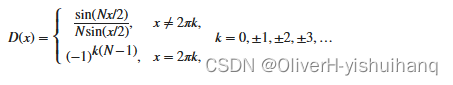
其中 N 是用户指定的正整数。如果 N 为奇数,则 Dirichlet 函数的周期为2π;如果 N 为偶数,则其周期为 4π。此函数的幅值是 1/N 乘以包含 N 个点的矩形窗的离散时间傅里叶变换的幅值。
要为 N=7 和 N=8 绘制 0 和 4π 之间的 Dirichlet 函数,使用:
figure
x = linspace(0,4*pi,300);

subplot(2,1,1)
plot(x/pi,diric(x,7))
title('N = 7')

subplot(2,1,2)
plot(x/pi,diric(x,8))
title('N = 8')
xlabel('x / \pi')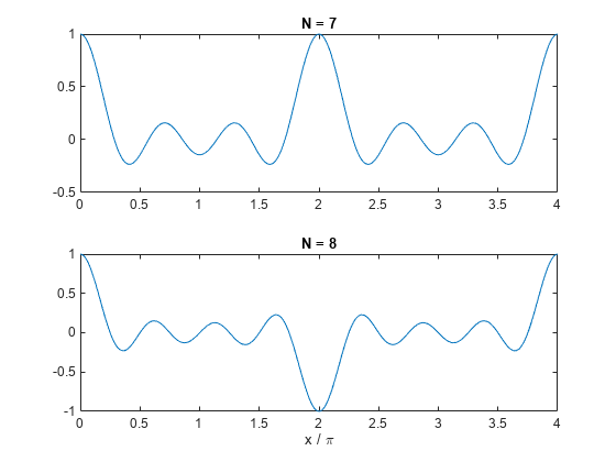
另请参阅
chirp | gauspuls | pulstran | rectpuls | sawtooth | sin | sinc | square | tripuls | vco
【我是小蜜蜂,知识的搬运工!】


 3533
3533

 被折叠的 条评论
为什么被折叠?
被折叠的 条评论
为什么被折叠?
 到【灌水乐园】发言


