英特尔 oneAPI 2023 黑客松大赛：赛道二机器学习：预测淡水质量 实践分享

一、问题描述

淡水是我们最重要和最稀缺的自然资源之一，仅占地球总水量的 3%。它几乎触及我们日常生活的方方面面，从饮用、游泳和沐浴到生产食物、电力和我们每天使用的产品。获得安全卫生的供水不仅对人类生活至关重要，而且对正在遭受干旱、污染和气温升高影响的周边生态系统的生存也至关重要。
比赛地址：英特尔 oneAPI 2023 黑客松大赛：赛道二机器学习：预测淡水质量

二、解决方案

1、方案简述

我们围绕赛道提供的数据集进行了多个特征间的相互交互，构造了一批与预测目标淡水质量相关的特征，并围绕特征与目标间的关联表现进行特征筛选，利用英特尔® Modin 分发版提升pandas处理特征集的效率，得到了49维相关特征作为最终的入模特证。最后，利用英特尔® 架构优化的XGBoost模型进行二分类，以此对淡水是否可以安全饮用而被依赖淡水的生态系统所使用进行预测。

2、数据分析

预处理

由于本赛道只有一份离线数据集，同时数据量级足够，我们在处理数据之前将该数据集按照5：2.5：2.5的比例划分为训练集、验证集、测试集。划分出测试集仅在模型推理阶段时使用，能够有效防止数据穿越等问题的发生，并能够准确对模型关于预测目标的拟合效果进行评估。

特征类型处理

1、特征类型划分为离散、连续两类特征

# 划分类别特征, 数值特征
cat_cols, float_cols = [], ['Target']
for col in data.columns:
    if data[col].value_counts().count() < 50:
        cat_cols.append(col)
    else:
        float_cols.append(col)
print('离散特征：', cat_cols)
print('连续特征：', float_cols)

离散特征： [‘Color’, ‘Source’, ‘Month’, ‘Day’, ‘Time of Day’, ‘Target’]
连续特征： [‘Target’, ‘pH’, ‘Iron’, ‘Nitrate’, ‘Chloride’, ‘Lead’, ‘Zinc’, ‘Turbidity’, ‘Fluoride’, ‘Copper’, ‘Odor’, ‘Sulfate’, ‘Conductivity’, ‘Chlorine’, ‘Manganese’, ‘Total Dissolved Solids’, ‘Water Temperature’, ‘Air Temperature’]

2、针对离散特征，进行缺失值处理

# 查看缺失值情况
display(data[cat_cols].isna().sum())
missing=data[cat_cols].isna().sum().sum()
print("\nThere are {:,.0f} missing values in the data.".format(missing))
print('-' * 50)

由于离散变量缺失比例都在1%左右，所以我们将缺失类别当作单独一类进行处理。

cateEnc_dict = {}
for col in cat_cols:
    if col == label_col:
        continue
    if str(data[col].dtype) == 'object':
        data[col] = data[col].fillna("#B")
    else:
        data[col] = data[col].fillna(-1000)
        data[col] = data[col].astype('int64')
    cate_set = sorted(set(data[col]))
    cateEnc_dict[col] = cate_set
    data[col] = data[col].replace(dict(zip(cate_set, range(1, len(cate_set) + 1))))

事实上，十二个月份属于有序类别特征，如果单纯地映射数字会破坏掉这种有序性，这里针对月份进行单独映射。

# 将月份映射至数字1~12
months = ["January", "February", "March", "April", "May",
          "June", "July", "August", "September", "October",
          "November", "December"]
data['Month'] = data['Month'].replace(dict(zip(months, range(1, len(months) + 1))))
display(data['Month'].value_counts())

针对明显无序的类别特征Color和Source，我们对其进行独特编码处理。对于有序类别特征，我们不对其进行额外处理。

# 将无序类别特征进行独热编码

color_ohe = OneHotEncoder()
source_ohe = OneHotEncoder()

X_color = color_ohe.fit_transform(data.Color.values.reshape(-1, 1)).toarray()
X_source = source_ohe.fit_transform(data.Source.values.reshape(-1, 1)).toarray()
pickle.dump(color_ohe, open('../feat_data/color_ohe.pkl', 'wb'))     # 将编码方式保存在本地
pickle.dump(source_ohe, open('../feat_data/source_ohe.pkl', 'wb'))   # 将编码方式保存在本地

dfOneHot = pandas.DataFrame(X_color, columns=["Color_" + str(int(i)) for i in range(X_color.shape[1])])
data = pandas.concat([data, dfOneHot], axis=1)

dfOneHot = pandas.DataFrame(X_source, columns=["Source_" + str(int(i)) for i in range(X_source.shape[1])])
data = pandas.concat([data, dfOneHot], axis=1)

由于连续变量缺失比例也都在2%左右，所以我们通过统计每个连续类别对应的中位数对缺失值进行填充。

display(data[float_cols].isna().sum())
missing=data[float_cols].isna().sum().sum()
print("\nThere are {:,.0f} missing values in the data.".format(missing))

# 使用中位数填充连续变量每列缺失值
fill_dict = {}
for column in list(data[float_cols].columns[data[float_cols].isnull().sum() > 0]):
    tmp_list = list(data[column].dropna())
    # 平均值
    mean_val = sum(tmp_list) / len(tmp_list)

    # 中位数
    tmp_list.sort()
    mid_val = tmp_list[len(tmp_list) // 2]
    if len(tmp_list) % 2 == 0:
        mid_val = (tmp_list[len(tmp_list) // 2 - 1] + tmp_list[len(tmp_list) // 2]) / 2

    fill_val = mid_val

    # 填充缺失值
    data[column] = data[column].fillna(fill_val)
    fill_dict[column] = fill_val

特征分布分析

# 针对每个连续变量的频率画直方图
data[float_cols].hist(bins=50,figsize=(16,12))

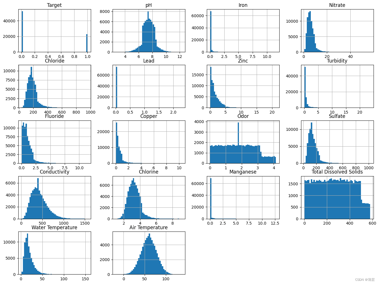
从上述直方图观察，有若干个变量的分布非常不规则，此处对它们进行非线性变换。

# 针对不规则分布的变量进行非线性变换，一般进行log
log_col = ['Iron', 'Zinc', 'Turbidity', 'Copper', 'Manganese']
show_col = []
for col in log_col:
    data[col + '_log'] = np.log(data[col])
    show_col.append(col + '_log')
    
# 特殊地，由于Lead变量0值占据了一定比例，此处特殊处理Lead变量
excep_col = ['Lead']
spec_val = {}
# 先将0元素替换为非0最小值，再进行log变换
for col in excep_col:
    spec_val[col] = data.loc[(data[col] != 0.0), col].min()
    data.loc[(data[col] == 0.0), col] = data.loc[(data[col] != 0.0), col].min()
    data[col + '_log'] = np.log(data[col])
    show_col.append(col + '_log')
    
data[show_col].hist(bins=50,figsize=(16,12))

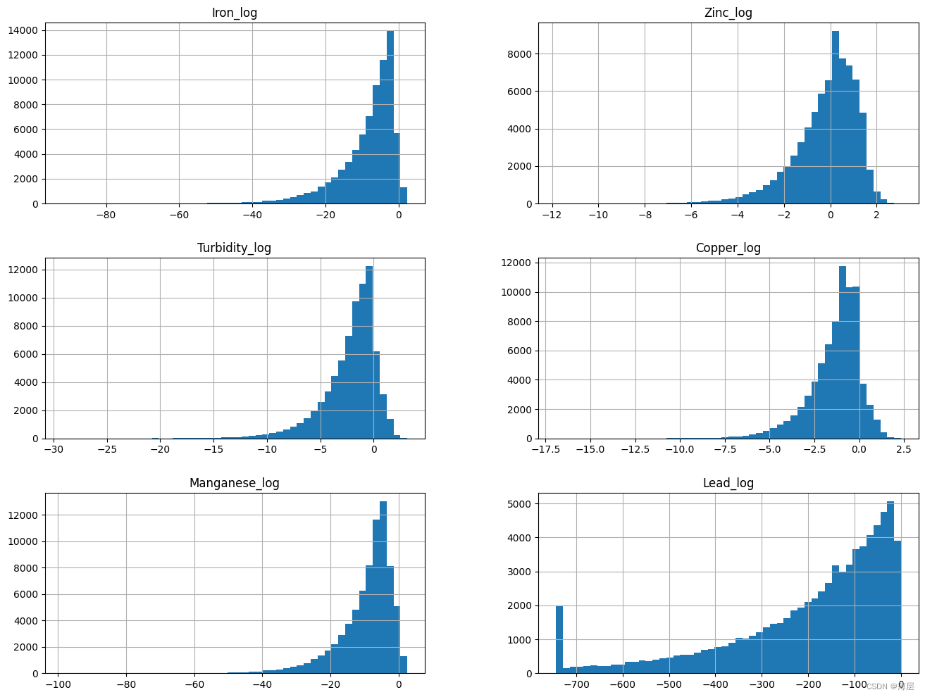
可以发现，上述不规则分布的变量经过log之后已经变成了模型更容易拟合的类正态分布。

3、特征构造

由于特征之间往往隐藏着很多相关的信息等待挖掘，此处进行特征关联，得到新的特征。由于时间关系，此处我们仅以类别特征进行分组，去依次统计其余特征在组内的中位数、均值、方差、最大值、最小值、计数特征，挖掘有效的交互特征。

# 特征交互统计
cat_interaction_dict = {}
del_feat_list = []
if 'del_feat_list' in count_fea_dict:
    del_feat_list = count_fea_dict['del_feat_list']
add_feat_list = []
    
for cat_col1 in cat_cols:
    if cat_col1 == label_col:
        continue
    new_col = cat_col1 + '_count'
    if new_col not in data.columns and new_col not in del_feat_list:
        add_feat_list.append(new_col)
        temp = data.groupby(cat_col1).size()
        cat_interaction_dict[new_col] = dict(temp)
        temp = temp.reset_index().rename(columns={0: new_col})
        data = data.merge(temp, 'left', on=cat_col1)
    for cat_col2 in cat_cols:
        if cat_col2 == label_col:
            continue
        if cat_col1 == cat_col2:
            continue
        new_col = cat_col1 + '_' + cat_col2 + '_count'
        if new_col not in data.columns and new_col not in del_feat_list:
            add_feat_list.append(new_col)
            temp = data.groupby(cat_col1)[cat_col2].nunique()
            cat_interaction_dict[new_col] = dict(temp)
            temp = temp.reset_index().rename(columns={cat_col2: new_col})
            data = data.merge(temp, 'left', on=cat_col1)

for cat_col in cat_cols:
    if cat_col == label_col:
        continue
    for float_col in float_cols:
        if float_col == label_col:
            continue

        new_col = cat_col + '_' + float_col + '_mean'
        if new_col not in data.columns and new_col not in del_feat_list:
            add_feat_list.append(new_col)
            temp = data.groupby(cat_col)[float_col].mean()
            cat_interaction_dict[new_col] = dict(temp)
            temp = temp.reset_index().rename(columns={float_col: new_col})
            data = data.merge(temp, 'left', on=cat_col)

        new_col = cat_col + '_' + float_col + '_median'
        if new_col not in data.columns and new_col not in del_feat_list:
            add_feat_list.append(new_col)
            temp = data.groupby(cat_col)[float_col].median()
            cat_interaction_dict[new_col] = dict(temp)
            temp = temp.reset_index().rename(columns={float_col: new_col})
            data = data.merge(temp, 'left', on=cat_col)

        new_col = cat_col + '_' + float_col + '_max'
        if new_col not in data.columns and new_col not in del_feat_list:
            add_feat_list.append(new_col)
            temp = data.groupby(cat_col)[float_col].max()
            cat_interaction_dict[new_col] = dict(temp)
            temp = temp.reset_index().rename(columns={float_col: new_col})
            data = data.merge(temp, 'left', on=cat_col)

        new_col = cat_col + '_' + float_col + '_min'
        if new_col not in data.columns and new_col not in del_feat_list:
            add_feat_list.append(new_col)
            temp = data.groupby(cat_col)[float_col].min()
            cat_interaction_dict[new_col] = dict(temp)
            temp = temp.reset_index().rename(columns={float_col: new_col})
            data = data.merge(temp, 'left', on=cat_col)

        new_col = cat_col + '_' + float_col + '_std'
        if new_col not in data.columns and new_col not in del_feat_list:
            add_feat_list.append(new_col)
            temp = data.groupby(cat_col)[float_col].std()
            cat_interaction_dict[new_col] = dict(temp)
            temp = temp.reset_index().rename(columns={float_col: new_col})
            data = data.merge(temp, 'left', on=cat_col)

4、特征选择

过滤法

由于本次目标是对淡水质量是否可用进行二分类预测，所以我们针对包含构造特征的所有特征数据，对于离散特征，利用卡方检验判断特征与目标的相关性，对于连续特征，利用方差分析判断特征与目标的相关性，以此做特征集的第一轮筛选。

# 卡方检验对类别特征进行筛选
def calc_chi2(x, y):
    import pandas as pd
    import numpy as np
    from scipy import stats
    
    chi_value, p_value, def_free, exp_freq = -1, -1, -1, []
    tab = pd.crosstab(x, y)
    if tab.shape == (2, 2):
        # Fisher确切概率法, 2✖️2列联表中推荐使用Fisher检验
        oddsr, p_value = stats.fisher_exact(tab, alternative='two-sided')
    else:
        # Pearson卡方检验, 参数correction默认为True
        chi_value, p_value, def_free, exp_freq = stats.chi2_contingency(tab, correction=False)

        min_exp = exp_freq.min()
        if min_exp >= 1 and min_exp < 5:
            # Yates校正卡方检验
            chi_value, p_value, def_free, exp_freq = stats.chi2_contingency(tab, correction=True)
    
    return chi_value, p_value, def_free, exp_freq

def select_feat_by_chi2(df, cate_cols, target_col, alpha=0.05, cut=99999):
    col_chi2_list = []
    for col in cate_cols:
        chi_value, p_value, def_free, exp_freq = calc_chi2(df[col], df[target_col])
        if p_value < alpha:
            col_chi2_list.append([col, chi_value])
    col_chi2_list = sorted(col_chi2_list, key=lambda x: x[1], reverse=False)
    rel_cols = []
    for i in range(min(len(col_chi2_list), cut)):
        rel_cols.append(col_chi2_list[i][0])
    return rel_cols
            
data = {
    'a': ['Ohio', 'Ohio', 'Ohio', 'Nevada', 'Nevada', 'Nevada'],
    'b': [2000, 2001, 2002, 2001, 2000, 2002],
    'Target': [0, 0, 1, 1, 1, 0]
}
df = pd.DataFrame(data)
cols = ['a', 'b']
select_feat_by_chi2(df, cols, 'Target')

# 方差分析法对连续特征进行筛选
def calc_fc(x, y):
    import pandas as pd
    import statsmodels.api as sm
    from statsmodels.formula.api import ols
    
    tab = pd.DataFrame({'group': y, 'feat': x})
    tab['group'] = tab['group'].astype('str').map(lambda x: 'g_' + x)

    mod = ols('feat ~ group', data=tab).fit()        
    ano_table = sm.stats.anova_lm(mod, typ=2)
    F = ano_table.loc['group', 'F']
    p_value = ano_table.loc['group', 'PR(>F)']
    return F, p_value

def select_feat_by_fc(df, cate_cols, target_col, alpha=0.05, cut=99999):
    from scipy import stats
    
    col_F_list = []
    for col in cate_cols:
        F, p_value = calc_fc(df[col], df[target_col])
        F_test = stats.f.ppf((1-alpha), 
                             df[target_col].nunique(),
                             len(df[col]) - df[target_col].nunique())
        # p值小于显著性水平 or MSa/MSe大于临界值，则拒绝原假设，认为各组样本不完全来自同一总体
        if p_value < alpha or F > F_test:
            col_F_list.append([col, F])
    col_F_list = sorted(col_F_list, key=lambda x: x[1], reverse=False)
    rel_cols = []
    for i in range(min(len(col_F_list), cut)):
        rel_cols.append(col_F_list[i][0])
    return rel_cols

data = {
    'a': [0.13, 0.09, 0.2, 0.11, 0.13, 0.15],
    'b': [2000, 2001, 2002, 2001, 2000, 2002],
    'Target': [0, 0, 1, 1, 1, 0]
}
df = pd.DataFrame(data)
cols = ['a', 'b']
select_feat_by_fc(df, cols, 'Target')

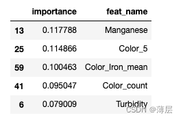
重要性排序

针对第一轮筛选剩余的150维特征，使用模型去进行拟合，并根据最后模型产出的特征重要性从大到小排序，根据重要性以及设定阈值对特征进行第二轮筛选。

# 模型训练函数
def train(data):
    ## Prepare Train and Test datasets ##
    print("Preparing Train and Test datasets")
    X_train, X_test, y_train, y_test = prepare_train_test_data(data=data,
                                                               target_col='Target',
                                                               test_size=.25)
    
    ## Initialize XGBoost model ##
    ratio = float(np.sum(y_train == 0)) / np.sum(y_train == 1)
    parameters = {
        'scale_pos_weight': len(raw_data.loc[raw_data['Target'] == 0]) / len(raw_data.loc[raw_data['Target'] == 1]),
        'objective': "binary:logistic", 
        'learning_rate': 0.1,
        'n_estimators': 18,
        'max_depth': 10,
        'min_child_weight': 5,
        'alpha': 4,
        'seed': 1024,
    }
    xgb_model = XGBClassifier(**parameters)
    xgb_model.fit(X_train, y_train)

    print("Done!\nBest hyperparameters:", grid_search.best_params_)
    print("Best cross-validation accuracy: {:.2f}%".format(grid_search.best_score_ * 100))
    
    ## Convert XGB model to daal4py ##
    xgb = grid_search.best_estimator_
    daal_model = d4p.get_gbt_model_from_xgboost(xgb.get_booster())

    ## Calculate predictions ##
    daal_prob = d4p.gbt_classification_prediction(nClasses=2,
                                                  resultsToEvaluate="computeClassLabels|computeClassProbabilities",
                                                  fptype='float').compute(X_test,
                                                                          daal_model).probabilities  # or .predictions
    xgb_pred = pd.Series(np.where(daal_prob[:, 1] > .5, 1, 0), name='Target')
    xgb_acc = accuracy_score(y_test, xgb_pred)
    xgb_auc = roc_auc_score(y_test, daal_prob[:, 1])
    xgb_f1 = f1_score(y_test, xgb_pred)

    ## Plot model results ##
    print("\ndaal4py Test ACC: {:.2f}%, F1 Accuracy: {:.2f}%, AUC: {:.5f}".format(xgb_acc * 100, xgb_f1 * 100, xgb_auc))
    # plot_model_res(model_name='XGBoost', y_test=y_test, y_prob=daal_prob[:, 1])

    importance_df = pd.DataFrame({'importance':xgb.feature_importances_,'feat_name': data.drop('Target', axis=1).columns})
    importance_df = importance_df.sort_values(by='importance', ascending=False)
    
    return importance_df

importance_df = train(data)
display(importance_df.head())

针对现有的150维特征对XGB模型进行拟合，并针对输出的特征重要性得分进行排序，将小于阈值的特征进行过滤。

5、模型训练

针对经过两轮筛选得到的49维入模特征，使用RandomizedSearchCV对XGBoost的重要参数进行搜索，同时使用StratifiedKFold对模型效果进行交叉验证。

import modin.pandas as pd
from modin.config import Engine
Engine.put("dask")
# import pandas as pd

import os
import daal4py as d4p
from xgboost import XGBClassifier
import time
import warnings
import pandas
import json
import numpy as np
import seaborn as sns
import matplotlib.pyplot as plt
import matplotlib.colors
import plotly.io as pio
import plotly.express as px
import plotly.graph_objects as go
from plotly.subplots import make_subplots
from sklearn.preprocessing import OneHotEncoder

from sklearnex import patch_sklearn
patch_sklearn()

from sklearn.model_selection import train_test_split, StratifiedKFold, GridSearchCV, RandomizedSearchCV
from sklearn.preprocessing import RobustScaler, StandardScaler
from sklearn.metrics import make_scorer, recall_score, precision_score, accuracy_score, roc_auc_score, f1_score
from sklearn.metrics import roc_auc_score, roc_curve, auc, accuracy_score, f1_score
from sklearn.metrics import precision_recall_curve, average_precision_score
from sklearn.svm import SVC
from xgboost import plot_importance
import pickle

# 引入可视化函数

warnings.filterwarnings('ignore')
pio.renderers.default='notebook' # or 'iframe' or 'colab' or 'jupyterlab'
intel_pal, color=['#0071C5','#FCBB13'], ['#7AB5E1','#FCE7B2']

# # 以"layout"为key，后面实例为value创建一个字典
temp=dict(layout=go.Layout(font=dict(family="Franklin Gothic", size=12), height=500, width=1000))


def prepare_train_test_data(data, target_col, test_size):
    """
    Function to scale and split the data into training and test sets
    """
    scaler = StandardScaler()
    
    X = data.drop(target_col, axis=1)
    y = data[target_col]
    
    X_train, X_test, y_train, y_test = train_test_split(X, y, test_size=test_size, random_state=21)

    # 按列归一化数据特征分布到 均值0方差1
    X_train_scaled = scaler.fit_transform(X_train)
    pickle.dump(scaler, open('../feat_data/scaler.pkl', 'wb'))  # 将编码方式保存在本地
    X_test_scaled = scaler.transform(X_test)
    print("Train Shape: {}".format(X_train_scaled.shape))
    print("Test Shape: {}".format(X_test_scaled.shape))

    return X_train_scaled, X_test_scaled, y_train, y_test


def plot_model_res(model_name, y_test, y_prob):
    """
    Function to plot ROC/PR Curves and predicted target distribution
    """

    intel_pal = ['#0071C5', '#FCBB13']
    color = ['#7AB5E1', '#FCE7B2']

    ## ROC & PR Curve ##
    fpr, tpr, _ = roc_curve(y_test, y_prob)
    roc_auc = auc(fpr, tpr)
    precision, recall, _ = precision_recall_curve(y_test, y_prob)
    auprc = average_precision_score(y_test, y_prob)

    fig = make_subplots(rows=1, cols=2,
                        shared_yaxes=True,
                        subplot_titles=['Receiver Operating Characteristic<br>(ROC) Curve',
                                        'Precision-Recall Curve<br>AUPRC = {:.3f}'.format(auprc)])
    # np.linspace等分0~1的区间为11份
    fig.add_trace(go.Scatter(x=np.linspace(0, 1, 11), y=np.linspace(0, 1, 11),
                             name='Baseline', mode='lines', legendgroup=1,
                             line=dict(color="Black", width=1, dash="dot")), row=1, col=1)
    fig.add_trace(go.Scatter(x=fpr, y=tpr, line=dict(color=intel_pal[0], width=3),
                             hovertemplate='True positive rate = %{y:.3f}, False positive rate = %{x:.3f}',
                             name='AUC = {:.4f}'.format(roc_auc), legendgroup=1), row=1, col=1)
    fig.add_trace(go.Scatter(x=recall, y=precision, line=dict(color=intel_pal[0], width=3),
                             hovertemplate='Precision = %{y:.3f}, Recall = %{x:.3f}',
                             name='AUPRC = {:.4f}'.format(auprc), showlegend=False), row=1, col=2)
    fig.update_layout(template=temp, title="{} ROC and Precision-Recall Curves".format(model_name),
                      hovermode="x unified", width=900, height=500,
                      xaxis1_title='False Positive Rate (1 - Specificity)',
                      yaxis1_title='True Positive Rate (Sensitivity)',
                      xaxis2_title='Recall (Sensitivity)', yaxis2_title='Precision (PPV)',
                      legend=dict(orientation='v', y=.07, x=.45, xanchor="right",
                                  bordercolor="black", borderwidth=.5))
    fig.show()

    ## Target Distribution ##
    plot_df = pd.DataFrame.from_dict({'State 0': (len(y_prob[y_prob <= 0.5]) / len(y_prob)) * 100,
                                      'State 1': (len(y_prob[y_prob > 0.5]) / len(y_prob)) * 100},
                                     orient='index', columns=['pct'])
    fig = go.Figure()
    fig.add_trace(go.Pie(labels=plot_df.index, values=plot_df.pct, hole=.45,
                         text=plot_df.index, sort=False, showlegend=False,
                         marker=dict(colors=color, line=dict(color=intel_pal, width=2.5)),
                         hovertemplate="%{label}: <b>%{value:.2f}%</b><extra></extra>"))
    fig.update_layout(template=temp, title='Predicted Target Distribution', width=700, height=450,
                      uniformtext_minsize=15, uniformtext_mode='hide')
    fig.show()

# 模型训练函数
def train(data):
    ## Prepare Train and Test datasets ##
    print("Preparing Train and Test datasets")
    X_train, X_test, y_train, y_test = prepare_train_test_data(data=data,
                                                               target_col='Target',
                                                               test_size=.25)
    
    ## Initialize XGBoost model ##
    ratio = float(np.sum(y_train == 0)) / np.sum(y_train == 1)
    parameters = {
        'scale_pos_weight': len(raw_data.loc[raw_data['Target'] == 0]) / len(raw_data.loc[raw_data['Target'] == 1]),
        'objective': "binary:logistic", 
        'learning_rate': 0.1,
        'n_estimators': 18,
        'max_depth': 10,
        'min_child_weight': 5,
        'alpha': 4,
        'seed': 1024,
    }
    xgb_model = XGBClassifier(**parameters)

    ## Tune hyperparameters ##
    strat_kfold = StratifiedKFold(n_splits=3, shuffle=True, random_state=21)
    print("\nTuning hyperparameters..")
    grid = {'min_child_weight': [1, 5, 10],
            'gamma': [0.5, 1, 1.5, 2, 5],
            'max_depth': [15, 17, 20],
            }

#     grid_search = RandomizedSearchCV(xgb_model, param_grid=grid,
#                                cv=strat_kfold, scoring=scorers,
#                                verbose=1, n_jobs=-1)
    
    strat_kfold = StratifiedKFold(n_splits=3, shuffle=True, random_state=1024)
    grid_search = RandomizedSearchCV(xgb_model, param_distributions=grid, 
                                    cv=strat_kfold, n_iter=10, scoring='accuracy', 
                                    verbose=1, n_jobs=-1, random_state=1024)
    grid_search.fit(X_train, y_train)

    print("Done!\nBest hyperparameters:", grid_search.best_params_)
    print("Best cross-validation accuracy: {:.2f}%".format(grid_search.best_score_ * 100))

    '''
    # normal predict ##
    xgb = grid_search.best_estimator_
    xgb_prob = xgb.predict_proba(X_test)[:, 1]
    xgb_pred = pd.Series(xgb.predict(X_test), name='Target')
    xgb_acc = accuracy_score(y_test, xgb_pred)
    xgb_auc = roc_auc_score(y_test, xgb_prob)
    xgb_f1 = f1_score(y_test, xgb_pred)

    print("\nTest ACC: {:.2f}%, F1 accuracy: {:.2f}%, AUC: {:.2f}%".format(xgb_acc * 100, xgb_f1 * 100, xgb_auc * 100))
    # print(xgb.feature_importances_)

    plot_model_res(model_name='XGB', y_test=y_test, y_prob=xgb_prob)
    '''
    
    ## Convert XGB model to daal4py ##
    xgb = grid_search.best_estimator_
    daal_model = d4p.get_gbt_model_from_xgboost(xgb.get_booster())

    ## Calculate predictions ##
    daal_prob = d4p.gbt_classification_prediction(nClasses=2,
                                                  resultsToEvaluate="computeClassLabels|computeClassProbabilities",
                                                  fptype='float').compute(X_test,
                                                                          daal_model).probabilities  # or .predictions
    xgb_pred = pd.Series(np.where(daal_prob[:, 1] > .5, 1, 0), name='Target')
    xgb_acc = accuracy_score(y_test, xgb_pred)
    xgb_auc = roc_auc_score(y_test, daal_prob[:, 1])
    xgb_f1 = f1_score(y_test, xgb_pred)

    ## Plot model results ##
    print("\ndaal4py Test ACC: {:.2f}%, F1 Accuracy: {:.2f}%, AUC: {:.5f}".format(xgb_acc * 100, xgb_f1 * 100, xgb_auc))
    # plot_model_res(model_name='XGBoost', y_test=y_test, y_prob=daal_prob[:, 1])

    ##
    importance_df = pd.DataFrame({'importance':xgb.feature_importances_,'feat_name': data.drop('Target', axis=1).columns})
    importance_df = importance_df.sort_values(by='importance', ascending=False)
    # pd.set_option('display.max_rows', None) #显示完整的行
    # display(importance_df.head())

    print('model saving...')
    pickle.dump(xgb, open("../result/model_best.dat", "wb"))
    
    return importance_df

训练得到最终模型后，对其进行保存，用于后续测试集的结果推理。

值得注意的一点是，针对测试集，需要根据训练集数据分布得到的统计值进行缺失值、独热编码等数据的处理，而非测试集数据分布下的统计值。最终，我们的模型在测试集上的ACC为89.04%。

总结

本项目在探索的过程中，先后经历了针对数据集进行精细化地特征分析、针对分析有效的数据特征进行特征交互，构建新的更有效的特征、针对特征工程后得到的408维特征，经过两轮特征选择得到49维高相关性特征，使用XGBoost进行模型训练，对最终模型进行多次拟合训练，得到了准确率在训练集表现88.76%，在验证集表现88.21%，在测试集表现89.04%的高准模型，同时在AUC评价下仍有很高的得分（测试集91.94%）。

未来工作

XGBoost虽然在训练阶段耗费不小的时间代价，但其在oneAPI提供的daal4py模型的加速下，其推理速度能得到更大的提升，随着数据量的增加，在保证训练机器足够的情况下，模型层面的准确率也会得到以进一步提升。

另外，我们的解决方案还有很大的提升空间，目前我们仅对少量的特征进行了分析以及交互处理，仍然有着很多潜在的与目标相关的信息等待着我们挖掘，相信在后续对本方案进行精细化探索后，仍然能够提升我们的模型性能。