一维卷积神经网络（1D-CNN）进行回归任务

import numpy as np
import pandas as pd
from sklearn.model_selection import train_test_split
from sklearn.preprocessing import StandardScaler
from tensorflow.keras.models import Sequential
from tensorflow.keras.layers import Conv1D, MaxPooling1D, Flatten, Dense, Activation, Dropout
from tensorflow.keras.optimizers import Adam
from tensorflow.keras.callbacks import Callback
from sklearn.metrics import mean_squared_error, mean_absolute_error, r2_score
import matplotlib.pyplot as plt

# Load the CSV data
file_path = 'data.csv'
data = pd.read_csv(file_path)

# Separate features and target variable
X = data.drop(columns=['VS'])
y = data['VS']

# Normalize the features
scaler = StandardScaler()
X_scaled = scaler.fit_transform(X)

# Split the data into training and testing sets
X_train, X_test, y_train, y_test = train_test_split(X_scaled, y, test_size=0.2, random_state=42)

# Reshape the data for CNN input
X_train_cnn = X_train.reshape(-1, X_train.shape[1], 1)
X_test_cnn = X_test.reshape(-1, X_test.shape[1], 1)

# Define the CNN model
model = Sequential()
model.add(Conv1D(64, kernel_size=3, activation='relu', input_shape=(X_train_cnn.shape[1], 1)))
model.add(Conv1D(64, kernel_size=3, activation='relu'))
model.add(MaxPooling1D(pool_size=2))
model.add(Flatten())
model.add(Dense(128, activation='relu'))
model.add(Dense(64, activation='relu'))
model.add(Dense(1))
model.add(Dense(32, activation='relu'))
model.add(Dense(1))
model.add(Dense(16, activation='relu'))
model.add(Dense(1))

# Compile the model
model.compile(optimizer=Adam(), loss='mean_squared_error')

# Define callbacks for training history
class History(Callback):
    def on_train_begin(self, logs={}):
        self.losses = {'batch': [], 'epoch': []}
        self.val_losses = {'batch': [], 'epoch': []}

    def on_batch_end(self, batch, logs={}):
        self.losses['batch'].append(logs.get('loss'))

    def on_epoch_end(self, epoch, logs={}):
        self.losses['epoch'].append(logs.get('loss'))
        self.val_losses['epoch'].append(logs.get('val_loss'))

history = History()

# Train the model
model.fit(X_train_cnn, y_train, epochs=200, batch_size=32,  callbacks=[history])

# Evaluate the model
y_pred = model.predict(X_test_cnn)
mse = mean_squared_error(y_test, y_pred)
mae = mean_absolute_error(y_test, y_pred)
r2 = r2_score(y_test, y_pred)

print('Test MSE:', mse)
print('Test MAE:', mae)
print(f'Test R^2: {r2:.4f}')

# Convert predictions and test data to original scale
y_test = y_test * (4426.3291 - 2609.2279) + 2609.2279
y_pred = y_pred * (4426.3291 - 2609.2279) + 2609.2279

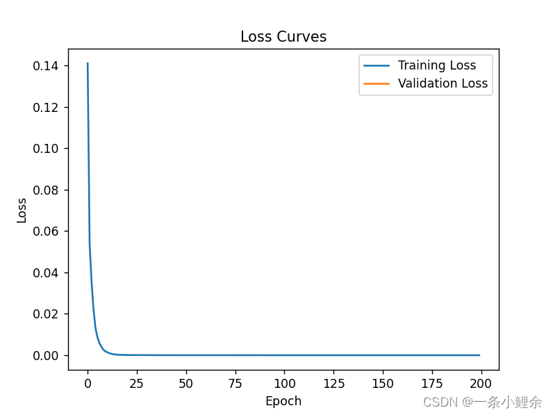
# Plot training and validation losses
plt.plot(history.losses['epoch'], label='Training Loss')
plt.plot(history.val_losses['epoch'], label='Validation Loss')
plt.xlabel('Epoch')
plt.ylabel('Loss')
plt.title('Loss Curves')
plt.legend()
plt.show()

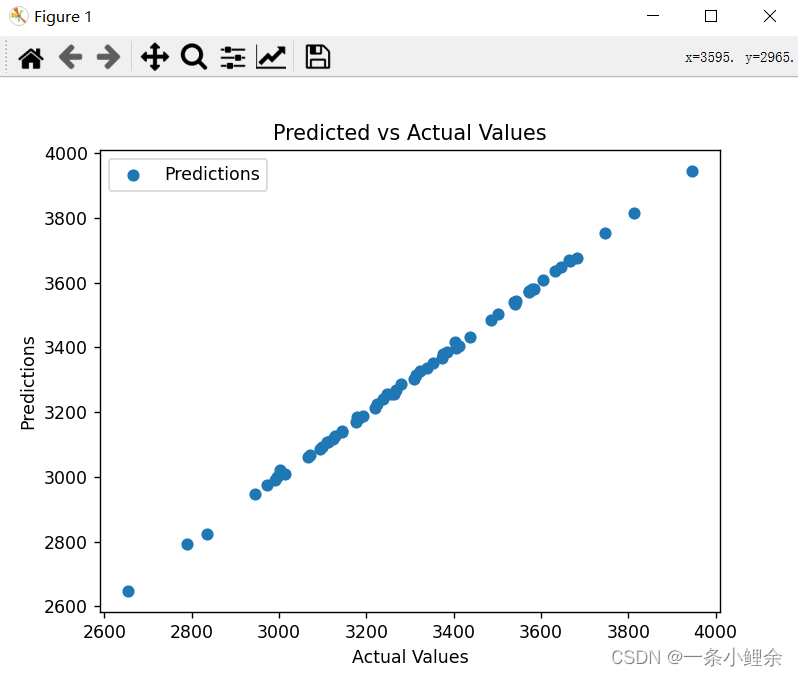
# Plot the predicted and actual values
plt.scatter(y_test, y_pred, label='Predictions')
plt.xlabel('Actual Values')
plt.ylabel('Predictions')
plt.title('Predicted vs Actual Values')
plt.legend()
plt.show()