线性回归算法（一）

最新推荐文章于 2024-02-18 23:03:13 发布

yumuluo

最新推荐文章于 2024-02-18 23:03:13 发布

阅读量233

点赞数

文章标签：线性回归算法回归

本文链接：https://blog.csdn.net/yumuluo/article/details/126570950

版权

（一）通俗解释：

①X1,X2就是我们的两个特征(年龄，工资)

Y是银行最终会借给我们多少钱

②找到最合适的一条线(想象一个高维)来，最好的拟合我们的数据点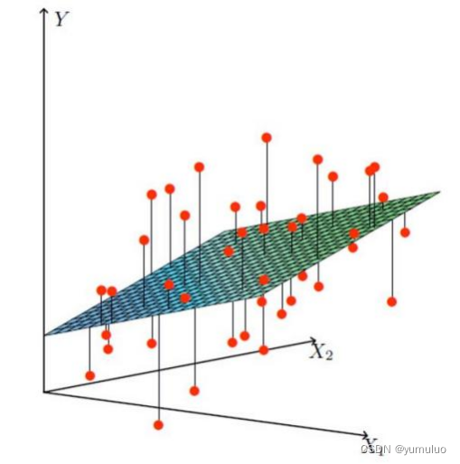

（二）数学来了：

1.假设θ1是年龄的参数，θ2是工资的参数

2.拟合的平面： $h_{\theta }(x) = \theta _{0} + \theta _{1}x_{1} + \theta _{2}x_{2}$ (θ0是偏置顶）

3.整合： $h_{\theta }(x) = \sum_{i = 0}^{n} \theta _{i}x_{i}= \theta {}^{T}x$

（三）误差：

1.真实值和预测值之间肯定是要存在差异的

(用 $\varepsilon$ 来表示该误差)

2.对于每个样本

$y^{(i)} = \theta ^{T}x^{(i)} + \varepsilon ^{(i)}$

(四）误差：

1.预测值与误差： $y^{(i)} = \theta ^{T}x^{(i)} + \varepsilon ^{(i)}$

2.由于误差服从高斯分布： $p(\epsilon ^{(i)}) = \frac{1}{\sqrt{2\Pi }\sigma }exp(\frac{\epsilon ^{(i)}\epsilon ^{(i)}}{2\sigma ^{2}})$

3.合并二式： $p(y^{(i)}|x^{(i)};\theta ) = \frac{1}{\sqrt{2\Pi }\sigma }exp(-\frac{(y^{(i)} - \theta ^{T}x^{(i)})^{2}}{2\sigma ^{2}})$

附上代码：

import numpy as np
from utils.features import prepare_for_training

class LinearRegression:

    def __init__(self,data,labels,polynomial_degree = 0,sinusoid_degree = 0,normalize_data=True):
        """
        1.对数据进行预处理操作
        2.先得到所有的特征个数
        3.初始化参数矩阵
        """
        (data_processed,
         features_mean, 
         features_deviation)  = prepare_for_training(data, polynomial_degree, sinusoid_degree,normalize_data=True)
         
        self.data = data_processed
        self.labels = labels
        self.features_mean = features_mean
        self.features_deviation = features_deviation
        self.polynomial_degree = polynomial_degree
        self.sinusoid_degree = sinusoid_degree
        self.normalize_data = normalize_data
        
        num_features = self.data.shape[1]
        self.theta = np.zeros((num_features,1))
        
    def train(self,alpha,num_iterations = 500):
        """
                    训练模块，执行梯度下降
        """
        cost_history = self.gradient_descent(alpha,num_iterations)
        return self.theta,cost_history
        
    def gradient_descent(self,alpha,num_iterations):
        """
                    实际迭代模块，会迭代num_iterations次
        """
        cost_history = []
        for _ in range(num_iterations):
            self.gradient_step(alpha)
            cost_history.append(self.cost_function(self.data,self.labels))
        return cost_history
        
        
    def gradient_step(self,alpha):    
        """
                    梯度下降参数更新计算方法，注意是矩阵运算
        """
        num_examples = self.data.shape[0]
        prediction = LinearRegression.hypothesis(self.data,self.theta)
        delta = prediction - self.labels
        theta = self.theta
        theta = theta - alpha*(1/num_examples)*(np.dot(delta.T,self.data)).T
        self.theta = theta
        
        
    def cost_function(self,data,labels):
        """
                    损失计算方法
        """
        num_examples = data.shape[0]
        delta = LinearRegression.hypothesis(self.data,self.theta) - labels
        cost = (1/2)*np.dot(delta.T,delta)/num_examples
        return cost[0][0]
        
        
        
    @staticmethod
    def hypothesis(data,theta):   
        predictions = np.dot(data,theta)
        return predictions
        
    def get_cost(self,data,labels):  
        data_processed = prepare_for_training(data,
         self.polynomial_degree,
         self.sinusoid_degree,
         self.normalize_data
         )[0]
        
        return self.cost_function(data_processed,labels)
    def predict(self,data):
        """
                    用训练的参数模型，与预测得到回归值结果
        """
        data_processed = prepare_for_training(data,
         self.polynomial_degree,
         self.sinusoid_degree,
         self.normalize_data
         )[0]
         
        predictions = LinearRegression.hypothesis(data_processed,self.theta)
        
        return predictions