线性回归算法（二）

最新推荐文章于 2024-04-02 11:15:57 发布

yumuluo

最新推荐文章于 2024-04-02 11:15:57 发布

阅读量628

点赞数 1

文章标签：算法线性回归机器学习

本文链接：https://blog.csdn.net/yumuluo/article/details/126571535

版权

（五）误差

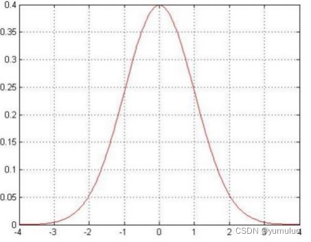
1.误差 $\varepsilon ^{(i)}$ 是独立并且具有相同的分布，并且服从均值为0方差为 $\theta ^{2}$ 的高斯分布

2.独立：张三和李四一起来贷款，他俩没关系

3. 同分布：他俩都来得是我们假定的这家银行

4.高斯分布：银行可能会多给，也可能会少给，但是绝大多数情况下这个浮动不会太大，极小情况下浮动会比较大，符合正常情况

(六）误差

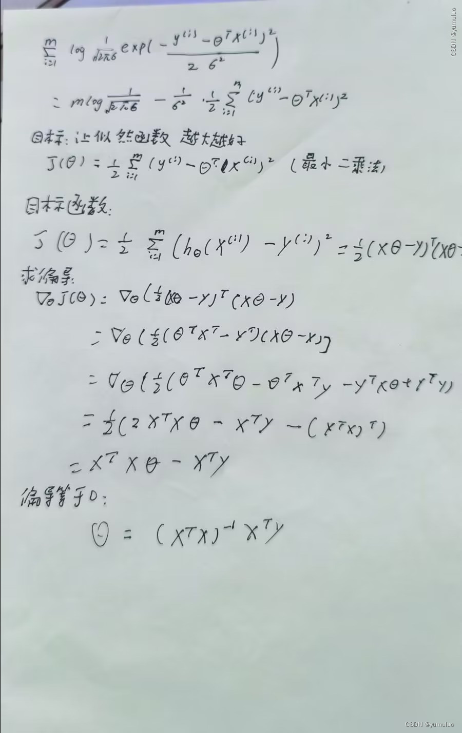
1.似然函数： $L = \prod_{i =1}^{m}$

解释：什么样的参数跟我们的数据组合后恰好是真实值

2.对数似然： $logL(\theta ) = long\prod_{i = 1}^{m}\frac{1}{\sqrt{2\Pi }\sigma }exp(-\frac{(y^{(i)} - \theta ^{T}x^{(i)})^{2}}{2\sigma ^{2}})$

解释：乘法难解，加法就容易了，对数里面乘法可以转换成加法

3.展开化简：

（七）评估方法

1.最常用的评估项 $R^{2}$ ：

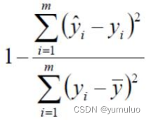
2. $R^{2}$ 的取值越接近1我们认为模型拟合的越好

全部代码：

import numpy as np
import pandas as pd
import matplotlib.pyplot as plt
import plotly
import plotly.graph_objs as go

plotly.offline.init_notebook_mode()
from linear_regression import LinearRegression

data = pd.read_csv('../data/world-happiness-report-2017.csv')

train_data = data.sample(frac=0.8)
test_data = data.drop(train_data.index)

input_param_name_1 = 'Economy..GDP.per.Capita.'
input_param_name_2 = 'Freedom'
output_param_name = 'Happiness.Score'


x_train = train_data[[input_param_name_1, input_param_name_2]].values
y_train = train_data[[output_param_name]].values

x_test = test_data[[input_param_name_1, input_param_name_2]].values
y_test = test_data[[output_param_name]].values

# Configure the plot with training dataset.
plot_training_trace = go.Scatter3d(
    x=x_train[:, 0].flatten(),
    y=x_train[:, 1].flatten(),
    z=y_train.flatten(),
    name='Training Set',
    mode='markers',
    marker={
        'size': 10,
        'opacity': 1,
        'line': {
            'color': 'rgb(255, 255, 255)',
            'width': 1
        },
    }
)


plot_test_trace = go.Scatter3d(
    x=x_test[:, 0].flatten(),
    y=x_test[:, 1].flatten(),
    z=y_test.flatten(),
    name='Test Set',
    mode='markers',
    marker={
        'size': 10,
        'opacity': 1,
        'line': {
            'color': 'rgb(255, 255, 255)',
            'width': 1
        },
    }
)


plot_layout = go.Layout(
    title='Date Sets',
    scene={
        'xaxis': {'title': input_param_name_1},
        'yaxis': {'title': input_param_name_2},
        'zaxis': {'title': output_param_name} 
    },
    margin={'l': 0, 'r': 0, 'b': 0, 't': 0}
)

plot_data = [plot_training_trace, plot_test_trace]

plot_figure = go.Figure(data=plot_data, layout=plot_layout)

plotly.offline.plot(plot_figure)

num_iterations = 500  
learning_rate = 0.01  
polynomial_degree = 0  
sinusoid_degree = 0  

linear_regression = LinearRegression(x_train, y_train, polynomial_degree, sinusoid_degree)

(theta, cost_history) = linear_regression.train(
    learning_rate,
    num_iterations
)

print('开始损失',cost_history[0])
print('结束损失',cost_history[-1])

plt.plot(range(num_iterations), cost_history)
plt.xlabel('Iterations')
plt.ylabel('Cost')
plt.title('Gradient Descent Progress')
plt.show()

predictions_num = 10

x_min = x_train[:, 0].min();
x_max = x_train[:, 0].max();

y_min = x_train[:, 1].min();
y_max = x_train[:, 1].max();


x_axis = np.linspace(x_min, x_max, predictions_num)
y_axis = np.linspace(y_min, y_max, predictions_num)


x_predictions = np.zeros((predictions_num * predictions_num, 1))
y_predictions = np.zeros((predictions_num * predictions_num, 1))

x_y_index = 0
for x_index, x_value in enumerate(x_axis):
    for y_index, y_value in enumerate(y_axis):
        x_predictions[x_y_index] = x_value
        y_predictions[x_y_index] = y_value
        x_y_index += 1

z_predictions = linear_regression.predict(np.hstack((x_predictions, y_predictions)))

plot_predictions_trace = go.Scatter3d(
    x=x_predictions.flatten(),
    y=y_predictions.flatten(),
    z=z_predictions.flatten(),
    name='Prediction Plane',
    mode='markers',
    marker={
        'size': 1,
    },
    opacity=0.8,
    surfaceaxis=2, 
)

plot_data = [plot_training_trace, plot_test_trace, plot_predictions_trace]
plot_figure = go.Figure(data=plot_data, layout=plot_layout)
plotly.offline.plot(plot_figure)

import numpy as np
import pandas as pd
import matplotlib.pyplot as plt

from linear_regression import LinearRegression

data = pd.read_csv('../data/non-linear-regression-x-y.csv')

x = data['x'].values.reshape((data.shape[0], 1))
y = data['y'].values.reshape((data.shape[0], 1))

data.head(10)

plt.plot(x, y)
plt.show()

num_iterations = 50000  
learning_rate = 0.02  
polynomial_degree = 15  
sinusoid_degree = 15  
normalize_data = True  

linear_regression = LinearRegression(x, y, polynomial_degree, sinusoid_degree, normalize_data)

(theta, cost_history) = linear_regression.train(
    learning_rate,
    num_iterations
)

print('开始损失: {:.2f}'.format(cost_history[0]))
print('结束损失: {:.2f}'.format(cost_history[-1]))

theta_table = pd.DataFrame({'Model Parameters': theta.flatten()})


plt.plot(range(num_iterations), cost_history)
plt.xlabel('Iterations')
plt.ylabel('Cost')
plt.title('Gradient Descent Progress')
plt.show()

predictions_num = 1000
x_predictions = np.linspace(x.min(), x.max(), predictions_num).reshape(predictions_num, 1);
y_predictions = linear_regression.predict(x_predictions)

plt.scatter(x, y, label='Training Dataset')
plt.plot(x_predictions, y_predictions, 'r', label='Prediction')
plt.show()

import numpy as np
import pandas as pd
import matplotlib.pyplot as plt

from linear_regression import LinearRegression

data = pd.read_csv('../data/world-happiness-report-2017.csv')

# 得到训练和测试数据
train_data = data.sample(frac = 0.8)
test_data = data.drop(train_data.index)

input_param_name = 'Economy..GDP.per.Capita.'
output_param_name = 'Happiness.Score'

x_train = train_data[[input_param_name]].values
y_train = train_data[[output_param_name]].values

x_test = test_data[input_param_name].values
y_test = test_data[output_param_name].values

plt.scatter(x_train,y_train,label='Train data')
plt.scatter(x_test,y_test,label='test data')
plt.xlabel(input_param_name)
plt.ylabel(output_param_name)
plt.title('Happy')
plt.legend()
plt.show()

num_iterations = 500
learning_rate = 0.01

linear_regression = LinearRegression(x_train,y_train)
(theta,cost_history) = linear_regression.train(learning_rate,num_iterations)

print ('开始时的损失：',cost_history[0])
print ('训练后的损失：',cost_history[-1])

plt.plot(range(num_iterations),cost_history)
plt.xlabel('Iter')
plt.ylabel('cost')
plt.title('GD')
plt.show()

predictions_num = 100
x_predictions = np.linspace(x_train.min(),x_train.max(),predictions_num).reshape(predictions_num,1)
y_predictions = linear_regression.predict(x_predictions)

plt.scatter(x_train,y_train,label='Train data')
plt.scatter(x_test,y_test,label='test data')
plt.plot(x_predictions,y_predictions,'r',label = 'Prediction')
plt.xlabel(input_param_name)
plt.ylabel(output_param_name)
plt.title('Happy')
plt.legend()
plt.show()