python——线性回归实例实战

最新推荐文章于 2024-04-08 11:09:48 发布

长沙有肥鱼

最新推荐文章于 2024-04-08 11:09:48 发布

阅读量3k

点赞数 2

分类专栏：机器学习文章标签： python 线性回归机器学习

本文链接：https://blog.csdn.net/weixin_53660567/article/details/123048523

版权

机器学习专栏收录该内容

11 篇文章 7 订阅

订阅专栏

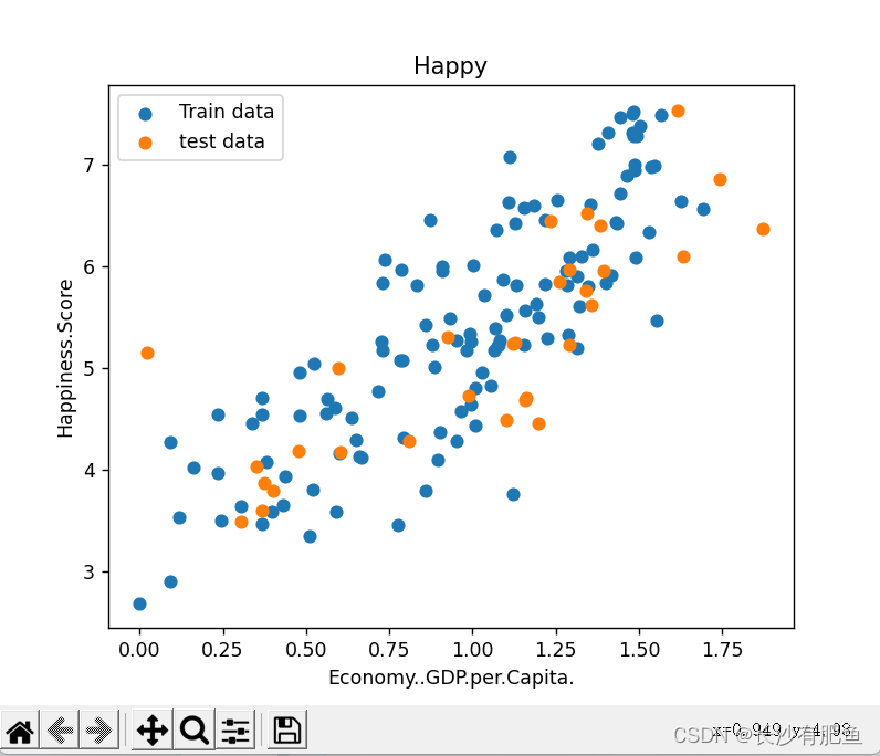
二维线性回归：

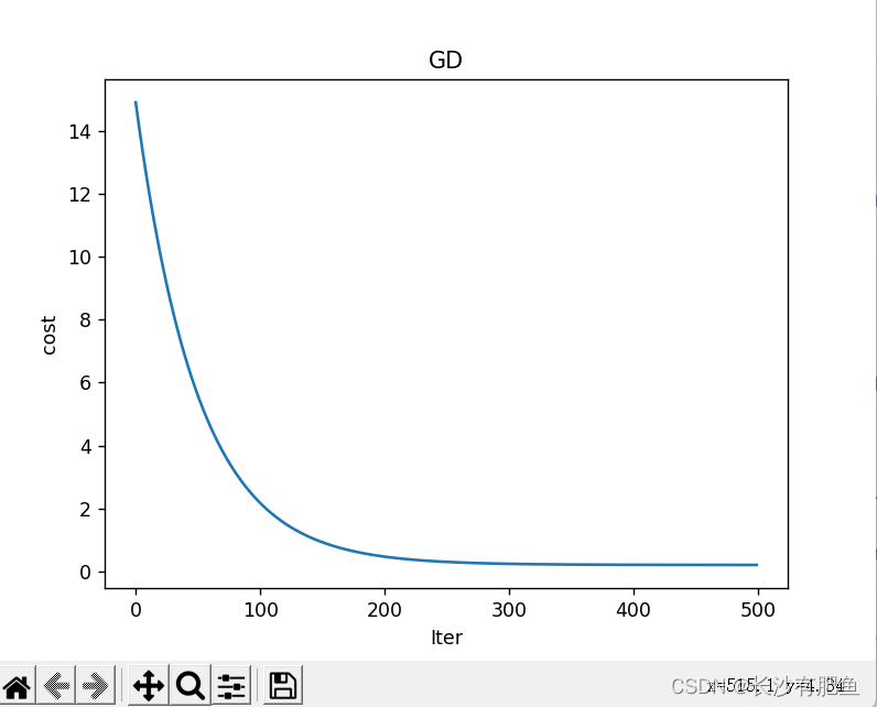
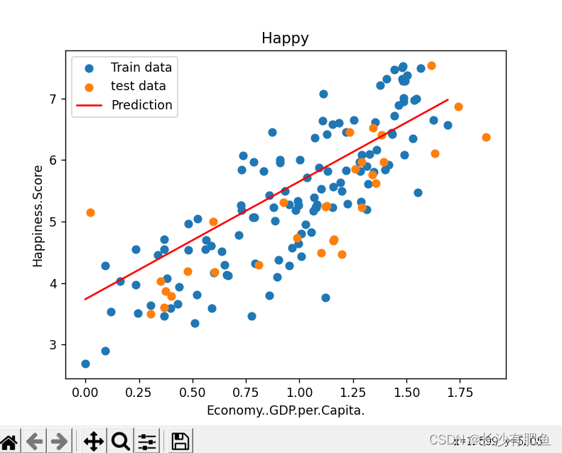
import numpy as np
import pandas as pd
import matplotlib.pyplot as plt

from linear_regression import LinearRegression

data = pd.read_csv('../data/world-happiness-report-2017.csv')

# 得到训练和测试数据
train_data = data.sample(frac = 0.8)
test_data = data.drop(train_data.index)

input_param_name = 'Economy..GDP.per.Capita.'
# 输入特征名字
output_param_name = 'Happiness.Score'
# 输出特征名字

x_train = train_data[[input_param_name]].values
# .values表示转换成ndarray格式 [input_param_name]表示列值
# shape = (124,1) min = 0.0226431842893362 max = 1.87076568603516
y_train = train_data[[output_param_name]].values
# .values表示转换成ndarray格式 [output_par  am_name]表示列值
# shape = (124,1) min = 2.90499997138977 max = 7.50400018692017
x_test = test_data[input_param_name].values
# x_test = [1.61646318 1.48238301 1.53570664 1.69227767 1.43092346 1.12786877, 1.43362653 1.3613559  1.41691518 1.09186447 0.72887063 1.21768391, 0.83375657 1.03522527 1.35593808 1.32087934 1.10180306 0.92557931, 0.95148438 0.78375626 0.47982019 0.36842093 1.15687311
# 31
y_test = test_data[output_param_name].values
# y_test =  [7.53700018 7.52199984 6.97700024 6.57200003 6.44199991 6.42399979, 6.42199993 6.16800022 5.92000008 5.87200022 5.83799982 5.82499981, 5.82299995 5.71500015 5.62099981 5.61100006 5.5250001  5.31099987, 5.27899981 5.07399988 4.96199989 4.70900011 4.69199991

# 散点图绘制
plt.scatter(x_train,y_train,label='Train data')
plt.scatter(x_test,y_test,label='test data')
plt.xlabel(input_param_name)
plt.ylabel(output_param_name)
plt.title('Happy')
plt.legend()
plt.show()

# 迭代次数
num_iterations = 500
# 学习率
learning_rate = 0.01

linear_regression = LinearRegression(x_train,y_train)
# data = {ndarray:(124,2)} labels = {ndarray:(124,1)} theta = {ndarray:(2,1)} [[5.30513794], [0.89649877]]
(theta,cost_history) = linear_regression.train(learning_rate,num_iterations)
# 调用train模块传入学习率和和迭代次数

print ('开始时的损失：',cost_history[0])
# cost_history[0]表示开始的
print ('训练后的损失：',cost_history[-1])
# cost_history[-1]表示最后的那次

# 梯度下降 损失函数
plt.plot(range(num_iterations),cost_history)
# x=range(num_iterations) y=cost_history
plt.xlabel('Iter')
plt.ylabel('cost')
plt.title('GD')
plt.show()

predictions_num = 100
x_predictions = np.linspace(x_train.min(),x_train.max(),predictions_num).reshape(predictions_num,1)
# .reshape(predictions_num,1) 表示100*1的矩阵再乘以  shape = (100, 1) min = 0.0226431842893362 max = 1.87076568603516
# x_train.min() -> 最小值,x_train.max() -> 最大值,predictions_num -> 数量
y_predictions = linear_regression.predict(x_predictions)
# shape = (100, 1) min = 3.7678074723211252 max = 6.84246841761371
plt.scatter(x_train,y_train,label='Train data')
plt.scatter(x_test,y_test,label='test data')
plt.plot(x_predictions,y_predictions,'r',label = 'Prediction')
# x值 y值 颜色
plt.xlabel(input_param_name)
plt.ylabel(output_param_name)
plt.title('Happy')
plt.legend()
plt.show()

多参数线性回归：

MultivariateLinearRegression.py

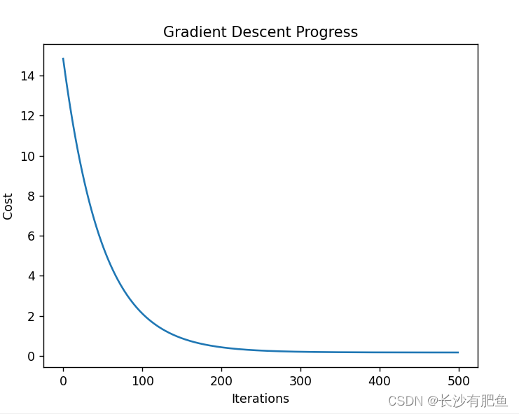
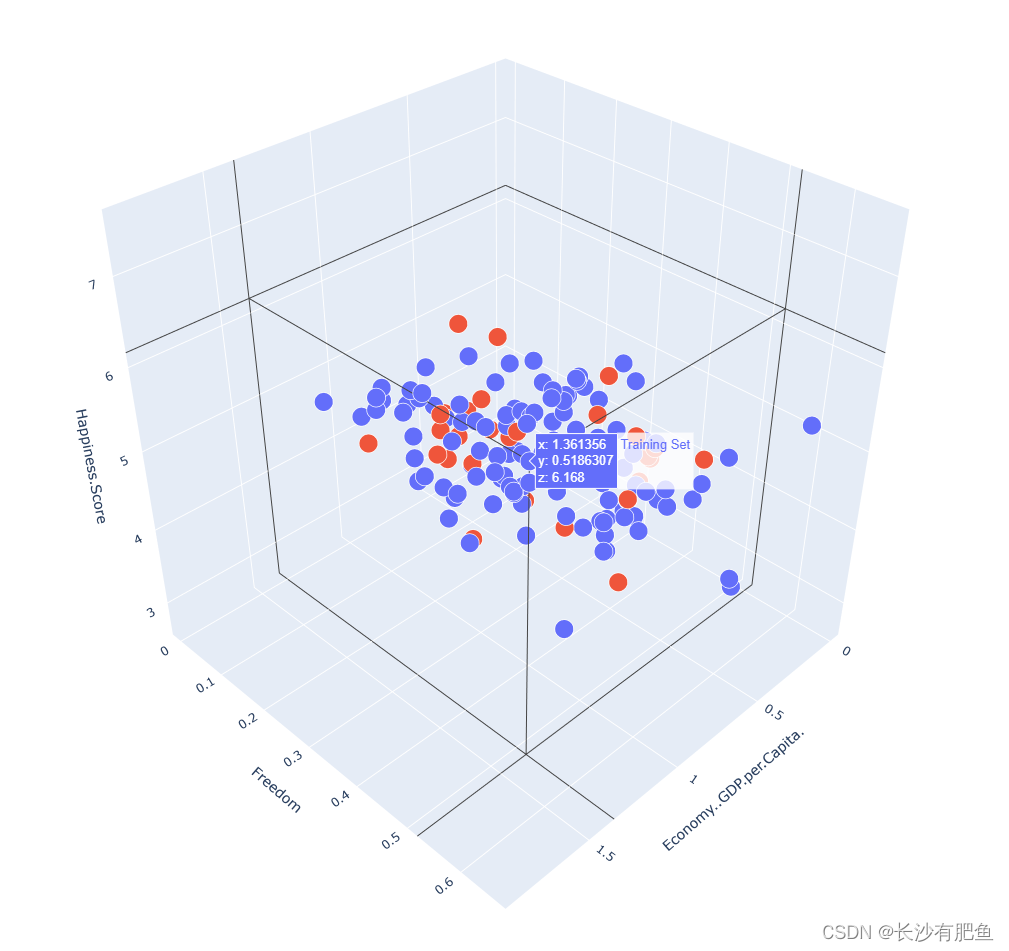
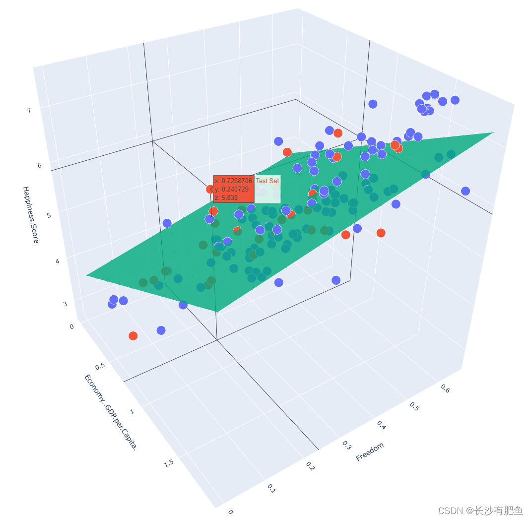
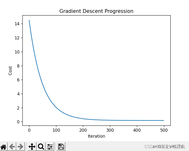
import numpy as np
import pandas as pd
import matplotlib.pyplot as plt
import plotly
import plotly.graph_objs as go
# https://plotly.com/python/line-and-scatter/
# https://plotly.com/python/
# plotly.offline.init_notebook_mode()
from linear_regression import LinearRegression

data = pd.read_csv('../data/world-happiness-report-2017.csv')
# Country  ...  Dystopia.Residual [0                      Norway  ...           2.277027] [1                     Denmark  ...           2.313707] [2                     Iceland  ...           2.322715] [3                 Switzerland  ...           2.276716]
# shape=(155, 12)
train_data = data.sample(frac=0.8)
# Country  ...  Dystopia.Residual [67         Libya  ...           1.835011] [9      Australia  ...           2.065211] [138      Lesotho  ...           1.429835] [110      Namibia  ...           1.481890] [66       Belarus  ...           1.723233] [..
# shape=(124, 12) 这里的shape值为155*9(frac=0.8)=124 其实就是将data中的一部分抽取出来当作训练数据
test_data = data.drop(train_data.index)
# shape=(31, 12)
# Country  ...  Dystopia.Residual [3    Switzerland  ...           2.276716] [5    Netherlands  ...           2.294804] [6         Canada  ...           2.187264] [10        Israel  ...           2.801757] [24        Mexico  ...           2.837155] [31

# x1 'Economy..GDP.per.Capita.'
input_param_name_1 = 'Economy..GDP.per.Capita.'
# x2 'Freedom'
input_param_name_2 = 'Freedom'
# y 'Happiness.Score'
output_param_name = 'Happiness.Score'


x_train = train_data[[input_param_name_1, input_param_name_2]].values
# [[1.10180306 0.46573323], [1.48441494 0.60160738], [0.52102125 0.3906613 ], [0.96443433 0.52030355], [1.15655756 0.29540026], [1.38439786 0.40878123], [0.77715313 0.08153944], [1.53062356 0.44975057], [0.79222125 0.469987  ], [1.43362653 0.36146659], [0.36
# 0.0  1.87076568603516 shape=(124, 2)
#  .values -> Return Series as ndarray or ndarray-like depending on the dtype.
y_train = train_data[[output_param_name]].values
# [[5.5250001 ], [7.28399992], [3.80800009], [4.57399988], [5.56899977], [6.40299988], [3.46199989], [6.34399986], [4.31500006], [6.42199993], [4.54500008], [5.26900005], [6.35699987], [6.99300003], [6.57200003], [5.82200003], [4.73500013], [4.51399994], [5.
# shape=(124, 1) min=2.69300007820129 max=7.53700017929077
x_test = test_data[[input_param_name_1, input_param_name_2]].values
# min=0.0149958552792668 max=1.56497955322266 shape=(31, 2)
y_test = test_data[[output_param_name]].values
# min=7.53700017929077 max=7.49399995803833 shape=(31, 1)
# Configure the plot with training dataset. Scatter3d三维散点图
plot_training_trace = go.Scatter3d(
    # :表示取所有数据 0表示取x1
    x=x_train[:, 0].flatten(),
    # [0.78644109 0.36874589 0.71624923 1.28601193 0.43801299 0.85769922, 0.88541639 1.44357193 0.30580869 1.12209415 0.78854758 1.48238301, 1.00726581 0.96443433 1.15360177 1.61646318 0.99553859 0.23430565, 0.60304892 1.40167844 1.34327984 0.73057312 1.48709726 0.59622008, 0.7372992  1.08116579 0.11904179 1.3613559  1.63295245 0.79222125, 0.47930902 1.10271049 1.43362653 1.2817781  0.98240942 1.39506662, 0.24454993 0.72887063 0.89465195 0.02264318 1.40570605 1.29178786, 1.2175597  1.62634337 0.9097845  1.87076569 0.56430537 1.10180306, 1.69227767 1.18529546 1.02723587 0.63640678 1.29121542 0., 0.90059674 1.49438727 0.23344204 1.46378076 0.09210235 1.10735321, 0.47618049 1.38439786 1.54625928 1.10970628 0.95148438 1.53570664, 1.15318382 1.16145909 1.19821024 1.1284312  1.15655756 1.18939555, 1.25278461 1.44163394 1.03522527 0.99619275 0.51113588 1.32087934, 1.28455627 0.93253732 0.80896425 1.09186447 0.35022771 1.07498753, 1.06931758 0.64845729 0.6017651  0.77715313 0.37584653 1.0008204, 1.2...
    # :表示取所有数据 0表示取x2
    y=x_train[:, 1].flatten(),
    # [0.65824866 0.58184385 0.25471106 0.17586352 0.16234203 0.58521467, 0.50153768 0.61795086 0.18919677 0.50519633 0.57105559 0.62600672, 0.28968069 0.52030355 0.39815584 0.63542259 0.44332346 0.48079109, 0.44770619 0.25792167 0.58876705 0.34807986 0.56776619 0.45494339, 0.44755185 0.47278771 0.33288118 0.51863074 0.49633759 0.469987, 0.37792227 0.28855553 0.36146659 0.37378311 0.20440318 0.25645071, 0.34858751 0.24072905 0.12297478 0.60212696 0.61406213 0.52034211, 0.57939225 0.60834527 0.43245253 0.60413098 0.43038875 0.46573323, 0.54984057 0.4945192  0.39414397 0.46160349 0.40226498 0.27084205, 0.19830327 0.6129241  0.46691465 0.53977072 0.23596135 0.43745375, 0.30661374 0.40878123 0.50574052 0.58013165 0.26028794 0.57311034, 0.41273001 0.28923172 0.31232858 0.15399712 0.29540026 0.49124733, 0.37689528 0.50819004 0.45000288 0.38149863 0.39001778 0.47913143, 0.43745428 0.47350779 0.43502587 0.23333581 0.32436785 0.28851599, 0.20871553 0.09609804 0.63337582 0.08153944 0.33638421 0.455198...
    z=y_train.flatten(),
    # [5.97100019 3.47099996 4.7750001  5.32399988 3.93600011 5.42999983, 5.01100016 7.46899986 3.64400005 3.76600003 5.07399988 7.52199984, 4.80499983 4.57399988 5.23400021 7.53700018 5.26200008 4.55000019, 4.17999983 5.83799982 6.52699995 5.18100023 7.00600004 5.00400019, 6.0710001  5.27299976 3.53299999 6.16800022 6.10500002 4.31500006, 4.53499985 4.49700022 6.42199993 5.96299982 5.18200016 5.96400023, 3.50699997 5.83799982 4.09600019 5.15100002 7.31400013 5.97300005, 6.454      6.64799976 6.00299978 6.375      4.69500017 5.5250001, 6.57200003 6.59899998 4.95499992 4.51399994 6.08400011 2.69300008, 4.37599993 7.28399992 3.97000003 6.89099979 4.28000021 6.63500023, 4.19000006 6.40299988 6.99300003 7.079      5.27899981 6.97700024, 6.57800007 4.71400023 4.46500015 5.25       5.56899977 5.62900019, 6.65199995 6.71400023 5.71500015 4.64400005 3.34899998 5.61100006, 5.81899977 5.49300003 4.29099989 5.87200022 4.03200006 5.2249999, 5.39499998 4.29199982 4.16800022 3.46199989 3.875      6.007999...
    name='Training Set',
    mode='markers',
    marker={
        'size': 10,
        'opacity': 1,
        'line': {
            'color': 'rgb(255, 255, 255)',
            # 颜色为红色
            'width': 1
        },
    }
)


plot_test_trace = go.Scatter3d(
    # [1.56497955 1.50394464 1.48441494 1.37538242 1.35268235 0.87200195, 1.53062356 1.41691518 1.26074862 1.21768391 0.83375657 1.13077676, 1.34120595 1.35593808 1.55167484 0.92557931 0.87811458 1.07937384, 1.31517529 1.06457794 0.52471364 0.47982019 1.05469871 0.36842093, 1.15687311 0.58668298 0.36711055 0.65951669 0.66722482 0.52102125, 0.36861026]
    x=x_test[:, 0].flatten(),
    # [0.62007058 0.58538449 0.60160738 0.4059886  0.49094617 0.53131062, 0.44975057 0.50562555 0.32570791 0.45700374 0.55873293 0.41827193, 0.57257581 0.35511154 0.49096864 0.47430724 0.40815833 0.55258983, 0.4984653  0.32590598 0.47156671 0.44030595 0.47924674 0.31869769, 0.24932261 0.47835666 0.51449203 0.01499586 0.42302629 0.3906613, 0.03036986]
    y=x_test[:, 1].flatten(),
    # [7.49399996 7.37699986 7.28399992 7.21299982 6.60900021 6.454, 6.34399986 5.92000008 5.8499999  5.82499981 5.82299995 5.82200003, 5.7579999  5.62099981 5.47200012 5.31099987 5.23500013 5.23000002, 5.19500017 5.17500019 5.04099989 4.96199989 4.829      4.70900011, 4.69199991 4.6079998  4.54500008 4.13899994 4.11999989 3.80800009, 3.60299993]
    z=y_test.flatten(),
    name='Test Set',
    mode='markers',
    marker={
        'size': 10,
        'opacity': 1,
        'line': {
            'color': 'rgb(255, 255, 255)',
            'width': 1
        },
    }
)


plot_layout = go.Layout(
    title='Date Sets',
    scene={
        # x轴
        'xaxis': {'title': input_param_name_1},
        # y轴
        'yaxis': {'title': input_param_name_2},
        # z轴
        'zaxis': {'title': output_param_name} 
    },
    margin={'l': 0, 'r': 0, 'b': 0, 't': 0}
)

plot_data = [plot_training_trace, plot_test_trace]

plot_figure = go.Figure(data=plot_data, layout=plot_layout)
# .Figure -> Create a new :class:Figure instance
plotly.offline.plot(plot_figure)

# 迭代次数
num_iterations = 500  
# 学习率
learning_rate = 0.01
polynomial_degree = 0
sinusoid_degree = 0  

linear_regression = LinearRegression(x_train, y_train, polynomial_degree, sinusoid_degree)
# data = {ndarray:(124,3)} [[ 1.00000000e+00 -4.41248542e-01  1.68691910e+00], [ 1.00000000e+00 -1.42201163e+00  1.18275714e+00], [ 1.00000000e+00 -6.06061512e-01 -9.75849221e-01], [ 1.00000000e+00  7.31761469e-01 -1.49612970e+00], [ 1.00000000e+00 -1.25937004e+00 -1.58535213e+00], [ 1.00000000e+00 -2.73931939e-01  1.20499972e+00], [ 1.00000000e+00 -2.08851037e-01  6.52851799e-01], [ 1.00000000e+00  1.10171790e+00  1.42101149e+00], [ 1.00000000e+00 -1.56979040e+00 -1.40814944e+00], [ 1.00000000e+00  3.46876726e-01  6.76993647e-01], [ 1.00000000e+00 -4.36302435e-01  1.11157012e+00], [ 1.00000000e+00  1.19284770e+00  1.47416863e+00], [ 1.00000000e+00  7.72557044e-02 -7.45099925e-01], [ 1.00000000e+00 -2.33141263e-02  7.76679555e-01], [ 1.00000000e+00  4.20857711e-01 -2.93198112e-02], [ 1.00000000e+00  1.50767269e+00  1.53629980e+00], [ 1.00000000e+00  4.97197916e-02  2.68721612e-01], [ 1.00000000e+00 -1.73768207e+00  5.15954124e-01], [ 1.00000000e+00 -8.71859835e-01  2.97641329e-01], [ 1.00000000e+00  1.00335052e+...
(theta, cost_history) = linear_regression.train(
    learning_rate,
    num_iterations
)
# theta shape=(3, 1) [[5.28604648], [0.80957372], [0.36349081]]
# cost_history  {list:500}
print('开始损失',cost_history[0])
print('结束损失',cost_history[-1])

plt.plot(range(num_iterations), cost_history)
plt.xlabel('Iterations')
plt.ylabel('Cost')
plt.title('Gradient Descent Progress')
plt.show()

predictions_num = 10

x_min = x_train[:, 0].min()
# x_min =0.0
x_max = x_train[:, 0].max()
# x_max = 1.87076568603516
y_min = x_train[:, 1].min()
# y_min = 0.0
y_max = x_train[:, 1].max()
# y_max = 0.658248662948608

x_axis = np.linspace(x_min, x_max, predictions_num)
# min= 0.0 max = 1.87076568603516  [0.         0.20786285 0.41572571 0.62358856 0.83145142 1.03931427, 1.24717712 1.45503998 1.66290283 1.87076569]
y_axis = np.linspace(y_min, y_max, predictions_num)
# min= 0.0 max = 0.658248662948608  [0.         0.07313874 0.14627748 0.21941622 0.29255496 0.3656937, 0.43883244 0.51197118 0.58510992 0.65824866]

x_predictions = np.zeros((predictions_num * predictions_num, 1))
# min= 0.0 max = 0.658248662948608 shape =(100,1)
y_predictions = np.zeros((predictions_num * predictions_num, 1))
# min= 0.0 max = 0.658248662948608  shape =(100,1)

x_y_index = 0
# x_y_index = 100
for x_index, x_value in enumerate(x_axis):
    # x_index:9 x_value:1.87076568603516
    for y_index, y_value in enumerate(y_axis):
        # y_index:9 y_value:0.658248662948608

        # 不断的得到x1
        x_predictions[x_y_index] = x_value
        # 不断的得到x2
        y_predictions[x_y_index] = y_value
        x_y_index += 1

z_predictions = linear_regression.predict(np.hstack((x_predictions, y_predictions)))
# shape = (100,1) min = 3.544753490888676 max = 6.9769309177100425
plot_predictions_trace = go.Scatter3d(
    x=x_predictions.flatten(),
    y=y_predictions.flatten(),
    z=z_predictions.flatten(),
    name='Prediction Plane',
    mode='markers',
    marker={
        'size': 1,
    },
    opacity=0.8,
    surfaceaxis=2, 
)

plot_data = [plot_training_trace, plot_test_trace, plot_predictions_trace]
plot_figure = go.Figure(data=plot_data, layout=plot_layout)
plotly.offline.plot(plot_figure)

梯度下降：

散点图：

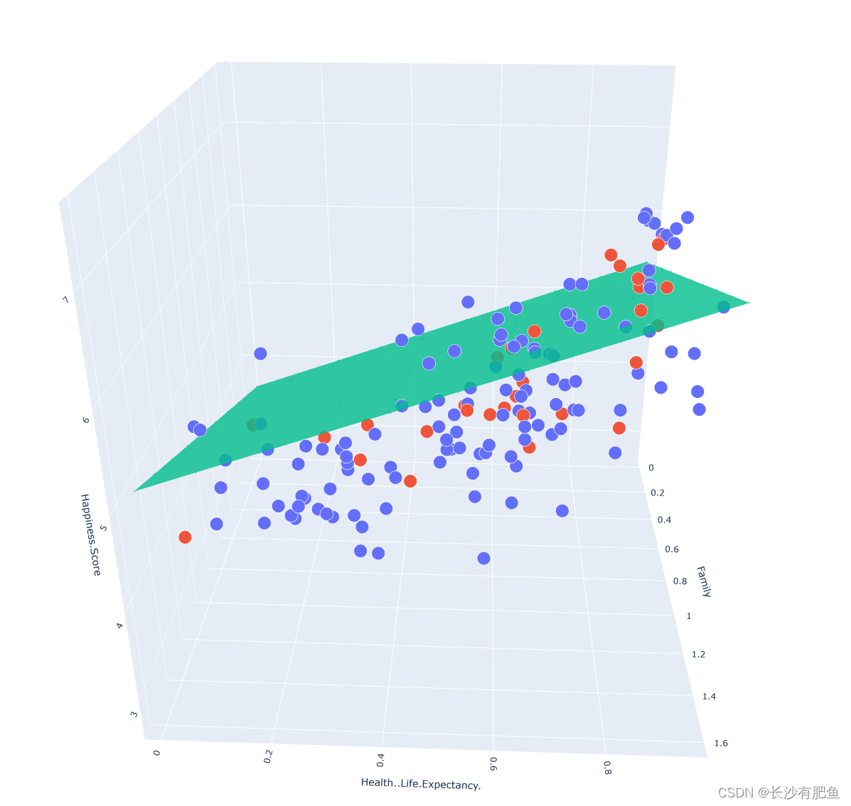
平面拟合：

开始损失 14.438348601809059
结束损失 0.22726258270086874

MultivariateLinearRegression1.py

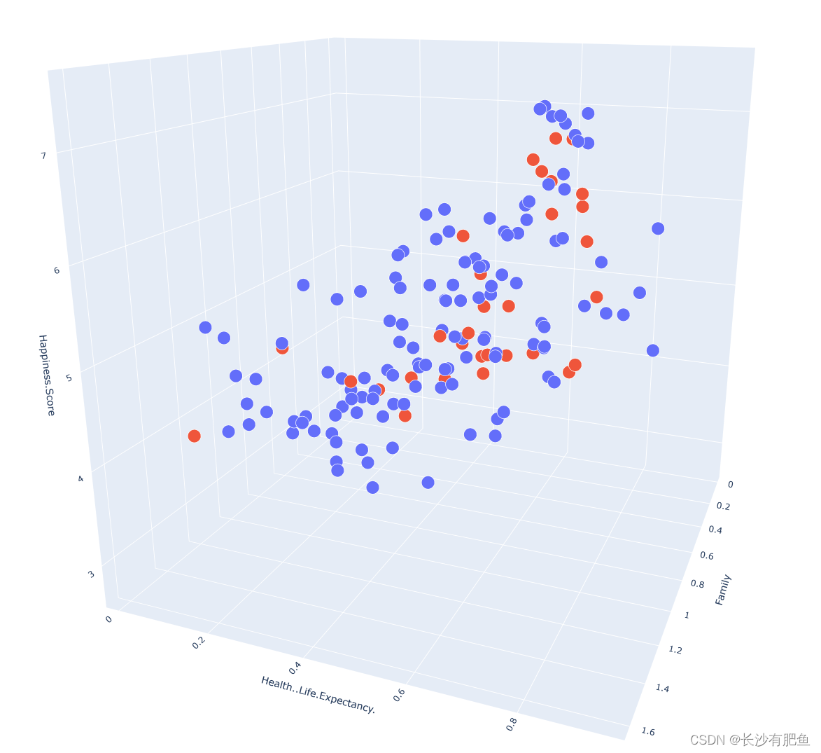
import numpy as np
import pandas as pd
import matplotlib.pyplot as plt
import plotly
import plotly.graph_objs as go

from linear_regression import LinearRegression

data = pd.read_csv('../data/world-happiness-report-2017.csv')

train_data = data.sample(frac=0.8)
test_data = data.drop(train_data.index)

input_param_name_1 = 'Family'
input_param_name_2 = 'Health..Life.Expectancy.'
output_param_name = 'Happiness.Score'

x_train = train_data[[input_param_name_1,input_param_name_2]].values
y_train = train_data[[output_param_name]].values

x_test = test_data[[input_param_name_1,input_param_name_2]].values
y_test = test_data[output_param_name].values

# 画出训练数据的三维散点图
plot_training_trace = go.Scatter3d(
    x=x_train[:, 0].flatten(),
    y=x_train[:, 1].flatten(),
    z=y_train.flatten(),
    name='Training set',
    mode='markers',
    marker={
        'size': 10,
        'opacity': 1,
        'line': {
            'color': 'rgb(255,255,255)',
            'width': 1
        },
    }
)

# 画出测试数据的三维散点图
plot_testing_trace = go.Scatter3d(
    x=x_test[:, 0].flatten(),
    y=x_test[:, 1].flatten(),
    z=y_test.flatten(),
    name='Testing set',
    mode='markers',
    marker={
        'size': 10,
        'opacity': 1,
        'line': {
            'color': 'rgb(255,255,255)',
            'width': 1
        },
    }
)

# 三维图的x轴,y轴,z轴的布局
plot_layout = go.Layout(
    title='Data Set',
    scene={
        'xaxis':{'title':input_param_name_1},
        'yaxis':{'title':input_param_name_2},
        'zaxis':{'title':output_param_name}
    },
    margin={'l':0,'r':0,'b':0,'t':0}
)

plot_data = [plot_training_trace,plot_testing_trace]
plot_figure = go.Figure(data=plot_data, layout=plot_layout)
plotly.offline.plot(plot_figure)

num_iterations = 500
learning_rate = 0.01
polynomial_degree = 0
sinusoid_degree = 0

linear_regression = LinearRegression(x_train,y_train,polynomial_degree,sinusoid_degree)
(theta,cost_history) = linear_regression.train(
    learning_rate,
    num_iterations
)
# 输出损失值
print('开始损失',cost_history[0])
print('结束损失',cost_history[-1])

# 画出损失函数
plt.plot(range(num_iterations),cost_history)
plt.xlabel('Iteration')
plt.ylabel('Cost')
plt.title('Gradient Descent Progression')
plt.show()

predictions_num = 10

x_min = x_train[:,0].min()
x_max = x_train[:,0].max()
y_min = x_train[:,1].min()
y_max = x_train[:,1].max()

x_axis = np.linspace(x_min,x_max,predictions_num)
y_axis = np.linspace(y_min,y_max,predictions_num)

x_predictions = np.zeros((predictions_num * predictions_num,1))
y_predictions = np.zeros((predictions_num * predictions_num,1))

x_y_index = 0
for x_index,x_value in enumerate(x_axis):
    for y_index,y_value in enumerate(y_axis):
        x_predictions[x_y_index] = x_value
        y_predictions[x_y_index] = y_value
        x_y_index += 1

z_predictions = linear_regression.predict(np.hstack((x_predictions,y_predictions)))
plot_predictions_trace = go.Scatter3d(
    x=x_predictions.flatten(),
    y=y_predictions.flatten(),
    z=z_predictions.flatten(),
    name='Prediction Plane',
    mode='markers',
    marker={
        'size': 1,
    },
    opacity=0.8,
    surfaceaxis=2,
)
plot_data = [plot_training_trace,plot_testing_trace,plot_predictions_trace]
plot_figure = go.Figure(data=plot_data,layout=plot_layout)
plotly.offline.plot(plot_figure)

非线性二维回归分析：

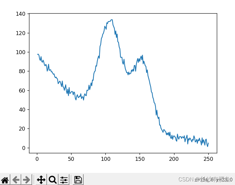
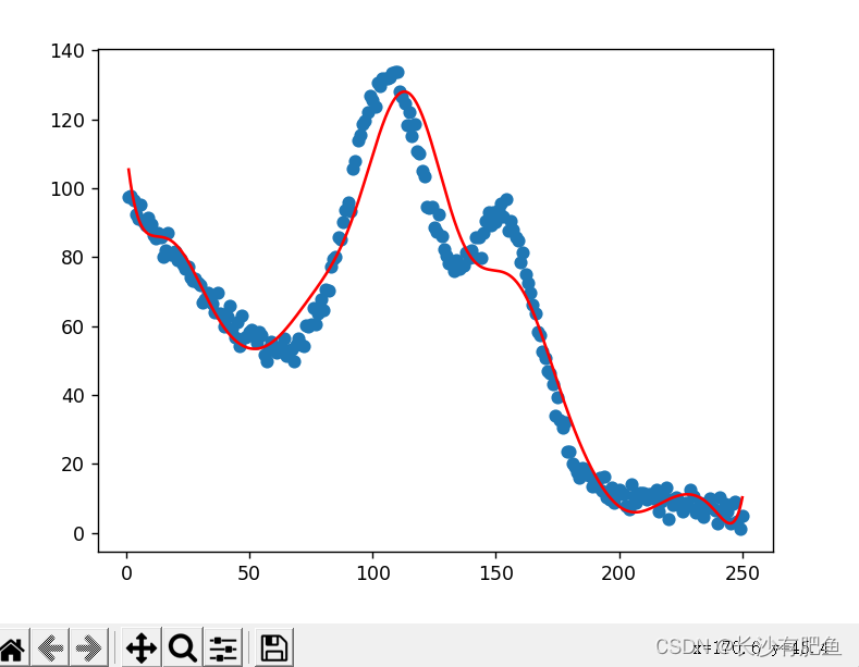
import numpy as np
import pandas as pd
import matplotlib.pyplot as plt

from linear_regression import LinearRegression
# 读取数据
data = pd.read_csv('../data/non-linear-regression-x-y.csv')

x = data['x'].values.reshape((data.shape[0], 1))
# shape=(250,1)
y = data['y'].values.reshape((data.shape[0], 1))
# shape=(250,1)
data.head(10)
# 画出曲线图
plt.plot(x, y)
plt.show()

# 迭代次数
num_iterations = 50000
# 学习率
learning_rate = 0.02
# 多项式
polynomial_degree = 15
# 对数据进行正弦计算
sinusoid_degree = 15  
normalize_data = True  

linear_regression = LinearRegression(x, y, polynomial_degree, sinusoid_degree, normalize_data)

(theta, cost_history) = linear_regression.train(
    learning_rate,
    num_iterations
)

print('开始损失: {:.2f}'.format(cost_history[0]))
print('结束损失: {:.2f}'.format(cost_history[-1]))

theta_table = pd.DataFrame({'Model Parameters': theta.flatten()})
# theta_table = {DataFrame:(152,1)}

plt.plot(range(num_iterations), cost_history)
plt.xlabel('Iterations')
plt.ylabel('Cost')
plt.title('Gradient Descent Progress')
plt.show()

predictions_num = 1000
x_predictions = np.linspace(x.min(), x.max(), predictions_num).reshape(predictions_num, 1)
# shape = (1000,1)
y_predictions = linear_regression.predict(x_predictions)
# y_predictions = {ndarray:(1000,1)}
plt.scatter(x, y, label='Training Dataset')
plt.plot(x_predictions, y_predictions, 'r', label='Prediction')
plt.show()

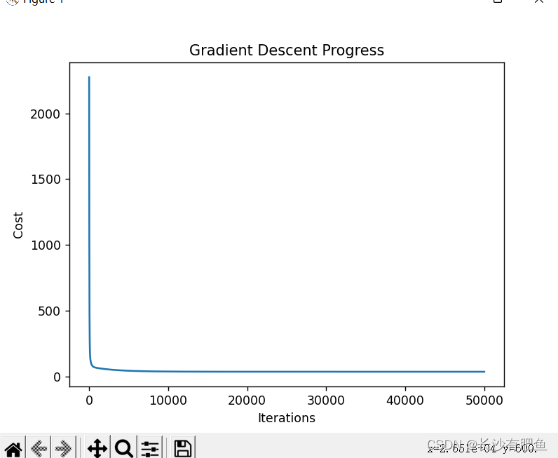
损失函数：

曲线拟合：

开始损失: 2274.66
结束损失: 35.04

长沙有肥鱼

关注

2
点赞
踩
33

收藏

觉得还不错? 一键收藏
打赏
6
评论
python——线性回归实例实战

MultivariateLinearRegression.pyimport numpy as npimport pandas as pdimport matplotlib.pyplot as pltimport plotlyimport plotly.graph_objs as go# https://plotly.com/python/line-and-scatter/# https://plotly.com/python/# plotly.offline.init_not...
复制链接

扫一扫