Dempster-Shafer Evidence Theory for Multimodality Classification

Dempster-Shafer Evidence Theory for Multimodality Classification

Author: Sijin Yu

*本文的举例、图片完全参考了 github 用户 Roy 的博客 [1]. 本文在其基础上增加了数学的形式化表达, 详细了其例, 重画了图片.

1. Discernment Frame (识别框架)

识别框架 (Discernment Frame) 指所有可能的基本事件的集合. 例如:
Θ = { θ 1 , θ 2 , ⋯   , θ n } \Theta =\{\theta_1,\theta_2,\cdots,\theta_n\} Θ={θ1​,θ2​,⋯,θn​}
就是一个由 $n$ 个两两互斥的基本事件构成的 discernment frame.

举例参考:

参考 [1] 中的举例, 考虑一个灯, 可能发出 R, G, B 三种颜色的光. 因此这里 $n=3$, 这三种基本事件为 ${\theta }_1=R$ 表示发红色光, ${\theta }_2=G$ 表示发绿色的光, ${\theta }_3=B$ 表示发绿色的光. 则 discernment frame 为 Θ = { θ 1 , θ 2 , θ 3 } = { R , G , B } \Theta =\{\theta_1, \theta_2, \theta_3\} =\{R, G, B\} Θ={θ1​,θ2​,θ3​}={R,G,B}.

2. Mass Function (质量函数)

给定 discernment frame $\Theta$, 质量函数 (Mass Function) 是定义在幂集 $2^{\Theta }$ 上的函数 $\mathcal{M}$, 定义为:
$$\mathcal{M}:2^{\Theta }\to [0,1]$$
Mass function $\mathcal{M}$ 满足两个性质,

• 空集的 mass 为 0, 即
  $$\mathcal{M}(\varnothing )=0$$

• 所有可能的组合的 mass 之和为 1, 即
  $$\sum _{A\subseteq \Theta }\mathcal{M}(A)=1$$

举例参考:

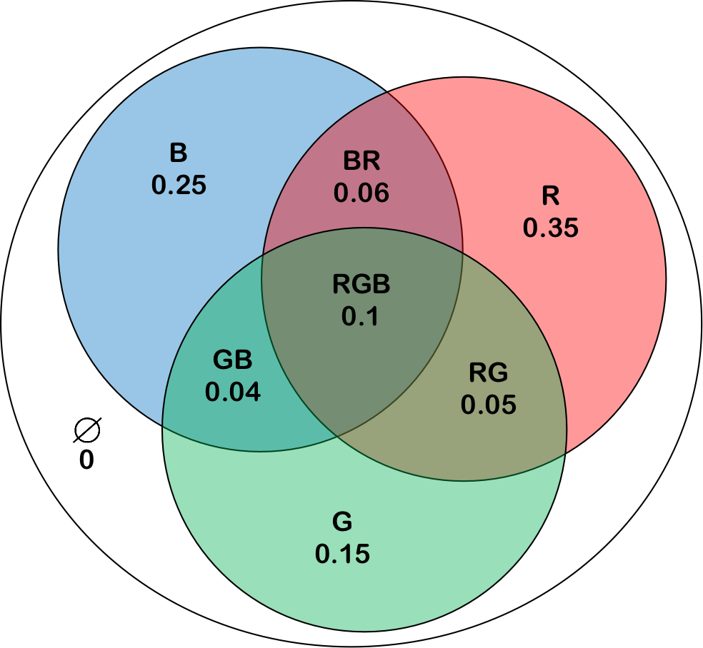
Mass 的意义是各种假设的可能性. 在上面的举例中, 假设一个观察者观测后, 对每个假设分配了 mass 值, 如下:

假设	含义	Mass
$\varnothing$	不发光	0
{ R } \{R\} {R}	发红光	0.35
{ G } \{G\} {G}	发绿光	0.15
{ B } \{B\} {B}	发蓝光	0.25
{ R , G } \{R, G\} {R,G}	发红光或绿光	0.05
{ G , B } \{G, B\} {G,B}	发绿光或蓝光	0.04
{ B , R } \{B, R\} {B,R}	发蓝光或红光	0.06
{ R , G , B } \{R, G, B\} {R,G,B}	发某一种光	0.1

画成 Venn Diagram 如下:

3. Belief Function (信度函数)

集合 $A\subseteq \Theta$ 的信度 (Belief) 定义为: $A$ 所有子集的 mass 之和. 即:
$$Bel(A)=\sum _{B\subseteq A}\mathcal{M}(B)$$

举例参考:

在上面的例子中, 各种组合的 belief 为:

• $Bel(R)=\mathcal{M}(R)=0.35$
• $Bel(G)=\mathcal{M}(G)=0.15$
• $Bel(B)=\mathcal{M}(B)=0.25$
• $Bel(RG)=\mathcal{M}(RG)+\mathcal{M}(R)+\mathcal{M}(G)=0.55$
• $Bel(GB)=\mathcal{M}(GB)+\mathcal{M}(G)+\mathcal{M}(B)=0.44$
• $Bel(BR)=\mathcal{M}(BR)+\mathcal{M}(B)+\mathcal{M}(R)=0.66$
• $Bel(RGB)=\mathcal{M}(RGB)+\mathcal{M}(RG)+\mathcal{M}(GB)+\mathcal{M}(BR)+\mathcal{M}(R)+\mathcal{M}(G)+\mathcal{M}(B)=1$

注意, 这里的数学符号不太严谨, 因为函数 $Bel(\cdot ),\mathcal{M}(\cdot )$ 的输入都是集合. 这里的 $Bel(R)$ 实际上应该为 B e l ( { R } ) Bel (\{R\}) Bel({R}), $\mathcal{M}(RGB)$ 实际上应该为 M ( { R , G , B } ) \mathcal M(\{R, G,B\}) M({R,G,B}), 其余同理. 这里采用这样的写法是为了简洁.

4. Plausibility Function (似然函数)

集合 $A\subseteq \Theta$ 的似然 (Plausibility) 定义为: 与 $A$ 相交的所有集合的 mass 之和. 即:
$$Pls(A)=\sum _{B\cap A\ne \varnothing }\mathcal{M}(B)$$

举例参考:

在上面的例子中, 各种组合的 plausibility 为:

• $Pls(R)=\mathcal{M}(R)+\mathcal{M}(RG)+\mathcal{M}(BR)+\mathcal{M}(RGB)=0.56$
• $Pls(G)=\mathcal{M}(G)+\mathcal{M}(RG)+\mathcal{M}(GB)+\mathcal{M}(RGB)=0.34$
• $Pls(B)=\mathcal{M}(B)+\mathcal{M}(GB)+\mathcal{M}(BR)+\mathcal{M}(RGB)=0.45$
• $Pls(RG)=\mathcal{M}(R)+\mathcal{M}(G)+\mathcal{M}(GB)+\mathcal{M}(BR)+\mathcal{M}(RG)+\mathcal{M}(RGB)=0.75$
• $Pls(GB)=\mathcal{M}(G)+\mathcal{M}(B)+\mathcal{M}(GB)+\mathcal{M}(BR)+\mathcal{M}(RG)+\mathcal{M}(RGB)=0.65$
• $Pls(BR)=\mathcal{M}(B)+\mathcal{M}(R)+\mathcal{M}(GB)+\mathcal{M}(BR)+\mathcal{M}(RG)+\mathcal{M}(RGB)=0.85$
• $Pls(RGB)=\mathcal{M}(R)+\mathcal{M}(G)+\mathcal{M}(B)+\mathcal{M}(GB)+\mathcal{M}(BR)+\mathcal{M}(RG)+\mathcal{M}(RGB)=1$

注意, 这里的数学符号不太严谨, 因为函数 $Pls(\cdot ),\mathcal{M}(\cdot )$ 的输入都是集合. 这里的 $Pls(R)$ 实际上应该为 P l s ( { R } ) Pls (\{R\}) Pls({R}), $\mathcal{M}(RGB)$ 实际上应该为 M ( { R , G , B } ) \mathcal M(\{R, G,B\}) M({R,G,B}), 其余同理. 这里采用这样的写法是为了简洁.

5. Probability Measure (概率测度)

给定 discernment frame $\Theta$, 概率测度 (Probability Measure) 是一个定义在集合 $\Theta$ 上的函数 $\mathcal{P}$, 定义为:
$$\mathcal{P}:\Theta \to [0,1]$$
Probability measure 满足以下性质:

• 归一性, 即:
  $$\sum _{\theta \in \Theta }\mathcal{P}(\theta )=1$$

• 可加性, 即:
  $$\mathcal{P}\left(\bigcup _i{\theta }_i\right)=\sum _i\mathcal{P}({\theta }_i)$$

  注意, 可加性的成立条件是 ${\theta }_{i_1},{\theta }_{i_2},\cdots ,{\theta }_{i_m}$ 为两两互斥的. 而这正是 discernment frame $\Theta$ 的定义给出的, 因此可加性自然成立.

  即然 ${\theta }_{i_1},{\theta }_{i_2},\cdots ,{\theta }_{i_m}(m\ge 2)$ 是两两互斥的, 因此下面的式子总成立:
  $$\mathcal{P}\left(\bigcap _i{\theta }_i\right)=0$$
  为了与我们上面使用 $RGB$ 表示 { R , G , B } \{R, G, B\} {R,G,B} 的符号保持一致性, 我们这里使用符号 $\mathcal{P}(RGB):=\mathcal{P}(R\cup G\cup B)$, 这与传统的 $\mathcal{P}(RGB)$ 表示 $\mathcal{P}(R\cap G\cap B)$ 不同 (后者在我们的例子中总是为 0, 没什么意思). 在这样的表述下, $\mathcal{P}(RG)$ 表示“该灯发红光或者发绿光”的概率测度, 其余的符号同理.

这里需要区分概率测度 $\mathcal{P}$ 和前面定义的质量函数 $\mathcal{M}$ 的区别.
$\mathcal{P}$ 的定义域是 $\Theta$, 即我们所理解的“概率”含义. $\mathcal{M}$ 的定义域是 $2^{\Theta }$, 它衡量了观测者对各种可能性判断的确定性 (这一解释在下文会再次说明).

6. 概率测度的界

任意一个子集 $A\subseteq \Theta$ 的概率测度定义为 $A$ 中元素之并的概率测度, 即
$$\mathcal{P}(A):=\mathcal{P}\left(\bigcup _{\theta \in A}\theta \right)=\sum _{\theta \in A}P(\theta )$$
其中, 第二个等式由 probability measure 的可加性给出.

$\mathcal{P}(A)$ 总是以 belief 为下界, 以 plausibility 为上界, 即:
$$Bel(A)\le \mathcal{P}(A)\le Pls(A)$$

7. Subjective Logic (主观逻辑)

使用主观逻辑 (Subjective Logic), 可以通过先验概率, 计算后验概率. 具体的, 若定义了 discernment frame $\Theta$, 在其上定义了 mass function $\mathcal{M}$, $\forall \theta \in \Theta$, 给定先验概率分布 $q(\theta )$, 则后验概率 $p(\theta )$ 可以如此得出:
p ( θ ) = M ( { θ } ) + ∑ θ ∈ A ⊆ Θ M ( A ) ⋅ q ( θ ∣ A ) p(\theta) = \mathcal M(\{\theta\}) +\sum_{\theta\in A\sube\Theta}\mathcal M(A)\cdot q(\theta|A) p(θ)=M({θ})+θ∈A⊆Θ∑​M(A)⋅q(θ∣A)

举例参考:

在上面的 RGB 灯例子中, 若给出先验概率分布如下:

$q(R)$	$q(G)$	$q(B)$
0.5	0.3	0.2

在上面 mass 分配的情况下, 可得修正的后验分布为:

$p(R)$	$p(G)$	$p(B)$
0.474	0.223	0.303

在上面的例子可见, mass 的数学意义是衡量不确定性, $\mathcal{M}(A)$ 即为分配给子集 $A$ 的证据 (Evidence).

8. Dempster-Shafer Evidence Combination (DS 证据合成)

假设有两个观察者, 它们观测的 mass function 分别为 ${\mathcal{M}}_1$ 和 ${\mathcal{M}}_2$.

${\mathcal{M}}_1$ 和 ${\mathcal{M}}_2$ 的冲突度 (Conflict Degree) $\gamma$ 定义如下:
$$\gamma =\sum _{A\cap B=\varnothing ,A,B\in \Theta }{\mathcal{M}}_1(A)\cdot {\mathcal{M}}_2(B)$$

冲突度衡量了 ${\mathcal{M}}_1$ 和 ${\mathcal{M}}_2$ 的不一致性.

• $\gamma \in [0,1]$ 总是成立.
• 若 $\gamma =0$, 表示两个证据源完全一致.
• 若 $\gamma =1$, 表示两个证据源完全冲突.

两个证据源的 mass function ${\mathcal{M}}_1$ 和 ${\mathcal{M}}_2$ 的正交和 (Orthogonal Sum) $\oplus$ 为融合后的 mass function $\mathcal{M}$. 具体的定义如下:
$$\mathcal{M}(A)={\mathcal{M}}_1\oplus {\mathcal{M}}_2(A):=\frac{1}{1-\gamma }\sum _{B\cap C=A}{\mathcal{M}}_1(B){\mathcal{M}}_2(C)$$

9. 用于多模态分类任务上的可能性

令 discernment frame $\Theta$ 的各元素定义为分类的各类别.

对于第 $i$ 个模态, 其 Encoder $E_i$ 处理这一模态的输入数据 $x_i$, 得到了对分类结果的先验分布 $q_i(\theta )$, $\forall \theta \in \Theta$. 同时, 使用一个模型去估计这个 Encoder 对分类结果的证据 mass function ${\mathcal{M}}_i(\theta )$, $\forall \theta \in \Theta$.

令可学习参数 ${\eta }_i\in [0,1]$ 用于衡量模态 $i$ 的可靠程度. 使用下面的方法更新 mass function ${\mathcal{M}}_i$:
$${\mathcal{M}}_i\leftarrow {\eta }_i{\mathcal{M}}_i+(1-{\eta }_i){\mathcal{M}}_{?}$$
这里, ${\mathcal{M}}_{?}$ 表示茫然的质量函数 (Vacuous Mass Function), 其定义为 ${\mathcal{M}}_{?}(\Theta )=1$.

使用 ${\eta }_i$ 对所有模态的先验分布做融合:
$$q(\theta )=\frac{1}{\sum {\eta }_i}\sum _i{\eta }_i{q}_i(\theta )$$
使用 DS Evidence Combination 对所有 mass function 做融合:
$$\mathcal{M}=\underset{i}{⨁}{\mathcal{M}}_i$$
最后, 使用 Subjective Logic 可以得到后验分布 $p(\theta )$ 为分类结果.

这种融合, 对多模态中存在某一模态可靠度不高, 但难以确定哪一模态可靠度不高, 需要模型自己学习每一模态的可靠度的情况, 有很大的促进意义. 此外, 这里的“多模态”也可以推广为“多分类器”、“多尺度”.

Reference List

[1] https://cf020031308.github.io/wiki/dempster-shafer-theory-and-subjective-logic/

[2] Shafer, G.: A mathematical theory of evidence, vol. 42. Princeton University Press (1976)