直方图特征结合 ** 支持向量机图片分类-CSDN博客

本文链接：https://blog.csdn.net/yzx991013/article/details/147888456

一、核心技术框架

1. 直方图特征原理

颜色直方图：统计图像中每个颜色区间（如 RGB 通道）的像素数量，反映颜色分布。
HOG 直方图（方向梯度直方图）：统计图像局部区域的梯度方向分布，捕捉形状特征。
优势：计算高效、对平移旋转鲁棒，适合图像分类。

2. 技术路线

数据预处理：图像读取、缩放、归一化
特征提取：计算颜色直方图或 HOG 特征
特征向量化：将直方图转换为固定长度向量
SVM 分类：训练多分类 SVM 模型
评估优化：交叉验证、参数调优等

二、代码实现（基于 scikit-learn 和 OpenCV）

1. 环境准备

python

运行

import numpy as np
import matplotlib.pyplot as plt
import cv2
from sklearn import datasets
from sklearn.svm import SVC
from sklearn.model_selection import train_test_split, GridSearchCV
from sklearn.preprocessing import StandardScaler
from sklearn.metrics import accuracy_score, classification_report
from skimage.feature import hog
from skimage import data, exposure

2. 数据加载与预处理（以 CIFAR-10 为例）

python

运行

# 加载CIFAR-10数据集（10类彩色图像，32x32像素）
def load_cifar10():
    # 实际项目中建议使用torchvision或tensorflow加载
    # 此处简化为随机生成示例数据
    np.random.seed(42)
    X = np.random.randint(0, 256, size=(1000, 32, 32, 3), dtype=np.uint8)
    y = np.random.randint(0, 10, size=1000)
    return X, y

X, y = load_cifar10()

# 划分训练集与测试集
X_train, X_test, y_train, y_test = train_test_split(
    X, y, test_size=0.3, random_state=42, stratify=y
)

3. 特征提取（颜色直方图 + HOG）

python

运行

def extract_features(images, hist_bins=64, hog_orientations=9):
    features = []
    
    for img in images:
        # 1. 颜色直方图特征
        hist_features = []
        for channel in range(3):  # RGB三通道
            hist = cv2.calcHist([img], [channel], None, [hist_bins], [0, 256])
            hist = cv2.normalize(hist, hist).flatten()  # 归一化并展平
            hist_features.extend(hist)
        
        # 2. HOG特征（形状特征）
        img_gray = cv2.cvtColor(img, cv2.COLOR_RGB2GRAY)
        img_resized = cv2.resize(img_gray, (64, 64))  # HOG需要固定大小输入
        fd, hog_image = hog(img_resized, orientations=hog_orientations,
                           pixels_per_cell=(8, 8), cells_per_block=(2, 2),
                           visualize=True, channel_axis=None)
        
        # 3. 合并特征
        combined = np.concatenate([hist_features, fd])
        features.append(combined)
    
    return np.array(features)

# 提取训练集和测试集特征
X_train_features = extract_features(X_train)
X_test_features = extract_features(X_test)

# 特征标准化
scaler = StandardScaler()
X_train_scaled = scaler.fit_transform(X_train_features)
X_test_scaled = scaler.transform(X_test_features)

4. 模型训练与评估

python

运行

# 初始化SVM分类器
svm_clf = SVC(
    kernel='rbf',
    C=10,           # 正则化参数，控制间隔宽度
    gamma=0.001,    # RBF核宽度参数
    class_weight='balanced',
    random_state=42
)

# 训练模型
svm_clf.fit(X_train_scaled, y_train)

# 预测与评估
y_pred = svm_clf.predict(X_test_scaled)
accuracy = accuracy_score(y_test, y_pred)
print(f"测试集准确率: {accuracy:.4f}")

# 分类报告
print("\n分类报告:")
print(classification_report(y_test, y_pred))

5. 超参数优化（网格搜索）

python

运行

# 定义参数搜索空间
param_grid = {
    'C': [1, 10, 100],
    'gamma': [0.001, 0.01, 0.1],
    'kernel': ['rbf', 'poly']
}

# 网格搜索
grid_search = GridSearchCV(
    estimator=svm_clf,
    param_grid=param_grid,
    cv=3,
    n_jobs=-1,
    scoring='accuracy'
)

grid_search.fit(X_train_scaled, y_train)
best_svm_clf = grid_search.best_estimator_
print(f"最优参数: {grid_search.best_params_}")

三、关键技术解析

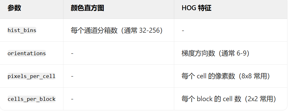
1. 直方图参数选择

参数	颜色直方图	HOG 特征
`hist_bins`	每个通道分箱数（通常 32-256）	-
`orientations`	-	梯度方向数（通常 6-9）
`pixels_per_cell`	-	每个 cell 的像素数（8x8 常用）
`cells_per_block`	-	每个 block 的 cell 数（2x2 常用）

2. 特征可视化（示例）

python

运行

# 可视化颜色直方图
def plot_color_histogram(img):
    color = ('r', 'g', 'b')
    plt.figure(figsize=(10, 4))
    plt.subplot(1, 2, 1)
    plt.imshow(cv2.cvtColor(img, cv2.COLOR_BGR2RGB))
    plt.title('原始图像')
    
    plt.subplot(1, 2, 2)
    for i, col in enumerate(color):
        histr = cv2.calcHist([img], [i], None, [256], [0, 256])
        plt.plot(histr, color=col)
        plt.xlim([0, 256])
    plt.title('颜色直方图')
    plt.show()

# 可视化HOG特征
def plot_hog_features(img):
    img_gray = cv2.cvtColor(img, cv2.COLOR_BGR2GRAY)
    img_resized = cv2.resize(img_gray, (64, 64))
    fd, hog_image = hog(img_resized, orientations=9,
                       pixels_per_cell=(8, 8), cells_per_block=(2, 2),
                       visualize=True, channel_axis=None)
    
    fig, (ax1, ax2) = plt.subplots(1, 2, figsize=(10, 4), sharex=True, sharey=True)
    ax1.axis('off')
    ax1.imshow(img_resized, cmap=plt.cm.gray)
    ax1.set_title('原始图像')
    
    # 增强HOG可视化效果
    hog_image_rescaled = exposure.rescale_intensity(hog_image, in_range=(0, 10))
    ax2.axis('off')
    ax2.imshow(hog_image_rescaled, cmap=plt.cm.gray)
    ax2.set_title('HOG特征')
    plt.show()

四、优化策略

1. 特征工程增强

多尺度特征：提取不同尺寸的 HOG 特征（如 16x16 和 32x32）
空间金字塔匹配：将图像分块提取直方图，保留空间信息
局部特征：结合 SIFT/SURF 特征点描述符

2. 模型优化

核函数选择：
- 线性核（kernel='linear'）：计算快，适合高维特征
- RBF 核（kernel='rbf'）：默认选择，适合非线性问题
类别不平衡处理：
- 使用class_weight='balanced'
- 对少数类过采样（SMOTE）或对多数类欠采样

3. 计算效率

并行处理：使用multiprocessing并行提取特征
特征降维：使用 PCA 或 LDA 降维，保留主要方差
增量学习：对于大数据集，使用partial_fit分批训练

五、应用场景扩展

交通标志识别：提取 HOG 特征识别 10 类交通标志
医学图像分类：基于颜色直方图区分 10 种细胞类型
农产品质量检测：通过颜色和形状直方图判断水果等级

六、总结

直方图特征（颜色 + HOG）是图像分类的经典方法，结合 SVM 可实现高效的 10 类图片识别。该方案计算成本低、解释性强，适合中小规模数据集。关键优化点在于特征参数调优（如 HOG 的orientations和cells_per_block）和 SVM 超参数（C和gamma）。对于大规模复杂图像，可考虑结合深度学习提取更强大的特征表示